Investigation 2.6: Healthy Body Temperatures (cont.)

Section 7.3 Investigation 2.6: Healthy Body Temperatures (cont.)

Reconsider the research question of Investigation 2.5 where a "one-sample \(t\)-test" found convincing evidence with a sample mean body temperature of \(\bar{x} = 98.249\)°F and a sample standard deviation of \(s = 0.733\)°F against the hypothesis that \(\mu = 98.6\) in the population of healthy adults. In fact, we were 95% confident that \(\mu\) actually fell between 98.122 and 98.376 degrees (so not all that far from 98.6) based on an estimated standard error of \(SE(\bar{x}) = 0.064\text{.}\)

🔗

Summary of Investigation 2.5 results showing confidence interval

Checkpoint 7.3.1. Interpret temperature concerns.

So if you recorded a body temperature of 98.6°F would you be convinced you were sick? What temperature values would you be concerned about?

🔗

Checkpoint 7.3.2. Apply Empirical Rule.

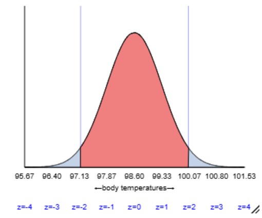
According to the Empirical Rule, if \(\mu = 98.6\)°F and \(\sigma = 0.733\)°F, between what two values should approximately 95% of healthy temperatures fall?

🔗

and

🔗

Solution.

\(98.249 \pm 2(0.733) = (96.783, 99.715)\text{.}\) We would expect approximately 95% of healthy human temperatures to fall in this interval.

🔗

Empirical Rule calculation showing 95% interval

🔗

Checkpoint 7.3.3. Compare to confidence interval.

Is your answer to Checkpoint 7.3.2 similar to the confidence interval from Checkpoint 7.2.24? Explain the difference in how the endpoints of the confidence interval are constructed and how we interpret the confidence interval.

🔗

Solution.

The interval in Checkpoint 7.3.2 is much wider than a 95% confidence interval. A 95% confidence interval would be \(98.249 \pm 1.96 (0.733/\sqrt{130}) = (98.12, 98.38)\text{.}\) This interval uses the sample size, and estimates the average human body temperature, not an individual body temperature. We are 95% confident the average human body temperature is between 98.12 and 98.38°F.

🔗

Prediction Intervals.

It is very important to keep in mind that the confidence interval reported above only makes statements about the population mean, not individual body temperatures. But what if we instead wanted an interval to estimate the body temperature of a single randomly selected healthy adult rather than the population mean body temperature? Can we improve upon the Empirical Rule calculation?

🔗

Checkpoint 7.3.4. Predict individual temperature.

Still using our same sample results, what one number would you use to predict a healthy body temperature? If you then considered the uncertainty (margin-of-error) in this estimate for predicting one person’s body temperature, would you expect this margin-of-error to be larger or smaller when predicting one person’s temperature than for predicting the population mean body temperature? Explain.

🔗

Estimate:

🔗

Margin-of-error comparison:

🔗

Solution.

We could still use the sample mean as the best one number prediction of a person’s healthy body temperature. But we would expect more uncertainty in this estimate of an individual person as there is a lot of person to person variation in body temperatures.

🔗

To construct such a confidence interval (often called a prediction interval to indicate that it will predict an individual outcome rather than the population mean), we need to consider both the sample-to-sample variation in sample means as well as the individual-to-individual variation in body temperatures around the mean.

🔗

\begin{equation*} \text{Var in temp} = \text{var in } \bar{x} + \text{var about } \bar{x} = \frac{s^2}{n} + s^2 \end{equation*}

🔗

Checkpoint 7.3.5. Compare standard errors.

We will estimate this combined standard error of an individual value by \(s\sqrt{1+\frac{1}{n}}\text{.}\) Using this formula, how will this compare to the standard error of the sample mean (larger or smaller)? Explain.

🔗

Smaller
Larger
The same

Hint.

Consider the extra \(1+\) under the square root.

🔗

Checkpoint 7.3.6. Calculate combined standard error.

Calculate \(s\sqrt{1+\frac{1}{n}}\) for the body temperature data.

🔗

Solution.

\(0.733\sqrt{1+\frac{1}{130}} \approx 0.735\)

🔗

If we are willing to assume that the population follows a normal distribution (note this is more restrictive than what we need to apply the Central Limit Theorem for a sample mean), then we can construct a 95% prediction interval for an individual outcome using the \(t\)-distribution.

🔗

Prediction Interval.

To predict an individual value, we can calculate a prediction interval (PI). We construct the interval using the sample mean as our estimate, but we adjust the standard error to take into account the additional variability of an individual value from the population mean:

🔗

\begin{equation*} \bar{x} \pm t_{n-1}^* s\sqrt{1+\frac{1}{n}} \end{equation*}

🔗

This procedure is valid as long as the sample observations are randomly selected from a normally distributed population. Note that prediction intervals are not robust to violations from the normality condition even with large sample sizes.

🔗

Aside: \(t\) Probability Calculator applet.

Checkpoint 7.3.7. Find \(t^*\) critical value.

Notice the critical value will be the same as in Checkpoint 7.2.23. Recall or use technology to determine the critical value with \(n = 130\) and 95% confidence.

🔗

\(t_{129}^*\) =

🔗

Solution.

\(t_{129}^* = 1.979\)

🔗

Checkpoint 7.3.8. Calculate prediction interval.

Using your answer to Checkpoint 7.3.7, calculate a 95% prediction interval for an individual healthy adult body temperature.

🔗

Solution.

95% prediction interval = \(98.249 \pm 1.979(0.735) = 98.249 \pm 1.455 = (96.79, 99.70)\)

🔗

JMP output showing prediction interval calculation

🔗

Checkpoint 7.3.9. Interpret prediction interval.

Provide a one-sentence interpretation of the interval calculated in Checkpoint 7.3.8.

🔗

Solution.

We are 95% confident that an individual randomly selected healthy adult will have a body temperature that is between 96.79°F to 99.71°F.

🔗

Checkpoint 7.3.10. Compare intervals.

(a) Center.

Center:

🔗

Smaller
The same
Larger

Hint.

Both intervals are centered at \(\bar{x}\text{.}\)

🔗

(b) Width.

Width:

🔗

Smaller
The same
Larger

Hint.

The prediction interval accounts for both sampling variability and individual variability.

🔗

Checkpoint 7.3.11. Compare to Empirical Rule interval.

How does this prediction interval compare to the interval from Checkpoint 7.3.2?

🔗

Solution.

The prediction interval is more similar to the answer from Checkpoint 7.3.2.

🔗

Checkpoint 7.3.12. Assess normality assumption.

The JAMA article only reported the summary statistics and did not provide the individual temperature values. If you had access to the individual data values, what could you do to assess whether the normality assumption is reasonable?

🔗

Solution.

To assess whether the normality assumption is reasonable, we can create a normal probability plot and judge whether the observations follow along the diagonal well. We can also look at a histogram.

🔗

Checkpoint 7.3.13. Evaluate plausibility of normality.

Without access to the individual data values but considering the context (body temperatures of healthy adults), do you have any thoughts about how plausible it is that the population is normally distributed?

🔗

Solution.

It is highly plausible that the population distribution is normally distributed because we would expect the majority of people to have a "regular" body temperature and fewer people who have body temperatures that are far from being regular.

🔗

Study Conclusions.

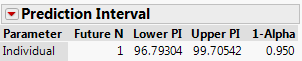
For one person to determine whether they have an unusual body temperature, we need a prediction interval rather than a confidence interval for the population mean. A 95% prediction interval for the body temperature of a healthy adult turns out to be (96.79, 99.71), a fairly wide interval. We are 95% confident that a randomly selected healthy adult will have a body temperature between 96.79 and 99.71 degrees Fahrenheit. This prediction interval procedure is valid only if the population of healthy body temperatures follows a normal distribution, which seems like a reasonable assumption in this context.

🔗

Exercises Practice Problem 2.6A

Examine the behavior of confidence intervals and prediction intervals as sample size increases.

🔗

1. Confidence interval width as \(n\) increases.

Examine the expression for a confidence interval for a population mean \(\bar{x} \pm t_{n-1}^* \frac{s}{\sqrt{n}}\text{.}\) What happens to the half-width of the interval as the sample size \(n\) increases? Does it approach a value as \(n\) increases?

🔗

2. Prediction interval width as \(n\) increases.

Examine the expression for a prediction interval for an individual observation \(\bar{x} \pm t_{n-1}^* s\sqrt{1+\frac{1}{n}}\text{.}\) What happens to the half-width of the interval as the sample size \(n\) increases? Does it approach a value as \(n\) increases?

🔗

3. Explain differences.

Explain why the differences in your answers to the previous two questions make sense.

🔗

Exercises Practice Problem 2.6B

A study conducted by Stanford researchers asked children in two elementary schools in San Jose, CA to keep track of how much television they watch per week (Robinson, 1999). The sample consisted of 198 children. The mean time spent watching television per week in the sample was 15.41 hours with a standard deviation of 14.16 hours.

🔗

1. Calculate prediction interval.

Use this information to calculate a 95% prediction interval.

🔗

2. Interpret prediction interval.

Provide a one-sentence interpretation of this interval.

🔗

3. Evaluate validity.

Do you think this interval procedure is valid for these data? Explain.

🔗

4. Compare to tolerance interval.

A tolerance interval claims to capture at least \(k\%\) of the population with \(C\%\) confidence. A 95% tolerance interval for these data with \(k = 95\) is (-14.95, 45.77). How does this interval compare to the prediction interval? Do these differences make sense? Explain.

🔗

You have attempted of activities on this page.

🔗

Prev Top Next