Section15.6Investigation 3.9: Smoking and Lung Cancer
In the previous investigation, you saw how to change the choice of statistic to relative risk. However, there are certain study designs where relative risk is not an appropriate choice, and so you will learn about another choice of statistic.
After World War II, evidence began mounting that there was a link between cigarette smoking and pulmonary carcinoma (lung cancer). In the 1950s, three now classic articles were published on the topic. One of these studies was conducted in the United States by Wynder and Graham ("Tobacco Smoking as a Possible Etiologic Factor in Bronchiogenic Cancer," 1950, Journal of the American Medical Association). They found records from a large number of patients with a specific type of lung cancer in hospitals in California, Colorado, Missouri, New Jersey, New York, Ohio, Pennsylvania, and Utah. Of those in the study, the researchers focused on 605 male patients with this form of lung cancer. Another 780 male hospital patients with similar age and economic distributions without this type of lung cancer were interviewed in St. Louis MO, Boston MA, Cleveland OH, and Hines IL. Subjects (or family members) were interviewed to assess their smoking habits, occupation, education, etc. The table below classifies them as a non-smoker or light smoker or as an at least a moderate smoker.
What is the estimate of the baseline rate of lung cancer from this table? Does that seem to be a reasonable estimate to you? How is this related to the design of the study? Explain.
Baseline risk ≈ 605/1385 = 0.437. It does not seem reasonable to believe that almost half of the population at that time was a lung cancer patient. This large proportion happens because the researchers controlled how many lung cancer and non-lung cancer patients would be in the study (and probably consciously trying to make them similar) rather than randomly selecting patients in general and seeing how many had lung cancer (recording the variable "naturally").
In the previous investigation, we found 3.4% of children in the sample had a peanut allergy. This seems like a reasonable estimate for the overall base rate because whether a child developed an allergy was observed "naturally," the frequency of those outcomes was in no way influenced by the researchers. However, in this study, the researchers had some control over the breakdown of lung cancer patients and control patients.
Cross-classification study: The researchers categorize subjects according to both the explanatory and the response variable simultaneously. For example, they could take a sample of adult males and simultaneously record both their smoking status and whether they have lung cancer. A common design is cross-sectional, where all observations are taken at a fixed point in time.
Cohort study: The researchers identify individuals according to the explanatory variable and then observe the outcomes of the response variable. These are usually prospective designs and may even follow the subjects (the cohort) for several years.
Case-control study: The researchers identify observational units in each response variable category (the "cases" and the "controls") and then determine the explanatory variable outcome for each observational unit. How the controls are selected is very important in determining the comparability of the groups. These are often retrospective designs in that the researchers may need to "look back" at historical data on the observational units.
This is a case-control study: the researchers found cases of lung cancer and then other similar patients without lung cancer (controls). Having lung cancer or not is the response variable.
An advantage of case-control studies is when you are studying a "rare event," you can ensure a large enough number of "successes" and fairly balanced group sizes. However, a disadvantage is that it does not make sense to calculate "risk" or likelihood of success from a case-control study, because the distribution of the response variable has been manipulated/determined by the researcher.
One alternative would be to calculate the relative risk of being in the heavy smoker group (which was observed naturally), comparing those with lung cancer to those without lung cancer (control).
The heavy smokers were 5.17 times more likely to have lung cancer compared to the light smokers. This value is not at all similar to the relative risk calculated in Question 3.
Switching the roles of the explanatory and response often gives very different results for relative risk (changing our measure of the strength of the relationship) and often really isn’t the comparison of interest stated by the research question. Consequently, conditional proportions of success and relative risk are not appropriate statistics to use with case-control studies. Instead, we will consider another way to compare the uncertainty of an outcome between two groups.
The odds of success are defined as the ratio of the proportion of "successes" to the proportion of "failures," which simplifies to the ratio of the number of successes to number of failures.
For example, if the odds are 2-to-1 in favor of an outcome, we expect a success twice as often as a failure in the long run, so this corresponds to a probability of 2/3 of the outcome occurring. Similarly, if the probability of success is 1/10, then the odds equals (1/10)/(9/10) = 1/9, and a failure is 9 times more likely than a success. It’s important to note how the "outcome" is defined. For example, in horse racing, odds are typically presented in terms of "losing the race," so if a horse is given 2-to-1 odds against winning a race, we expect the horse to lose two-thirds of the races in the long run.
Like relative risk, if the odds ratio is 3, this is interpreted as "the odds of success in the ’top’ group are 3 times (or 200%) higher than the odds of success in the ’bottom’ group." However, the relative risk and the odds ratio are not always similar in value.
Calculate and interpret the odds ratio comparing the odds of being a heavy smoker (rather than light smoker) for the lung cancer patients to the odds of being a heavy smoker in the control group. Does this match Question 3?
Calculate and interpret the odds ratio comparing the odds of lung cancer for the smokers to the odds of lung cancer for the nonsmokers. Does this match Question 4 or Question 5?
A major disadvantage to relative risk is that your (descriptive) measure of the strength of evidence that one group is "better" depends on which outcome you define a success as well as which variable you treat as the explanatory and which as the response. But a big advantage to odds ratio is that it is invariant to these definitions. (If your odds are 10 times higher to die from lung cancer if you are a smoker, then your odds of being a smoker are 10 times higher if you died from lung cancer). The only real disadvantage is that the odds ratio is trickier to interpret ("higher odds" vs. the more natural "more likely"). Thus, for case-control studies in particular, the odds ratio is the preferred statistic. However, when the success proportions are both small, the odds ratio can be used to approximate the relative risk.
So we could use either Odds Ratio as the statistic, we should just be consistent. Also notice that the odds of not having lung cancer are 1/9.39 = 0.106 times smaller for the light smokers than the heavy smokers.
Let \(\tau\) ("tau") represent the population odds ratio of being a heavy smoker comparing the population of lung cancer patients to the population of control patients, keeping in mind that this is equivalent to the population odds ratio of interest, but matches the study design, e.g.,
where \(\pi_1\) is probability of a lung cancer patient being a heavy smoker and \(\pi_2\) is the probability of a control patient being a heavy smoker.
Ha: \(\tau > 1\) (the population odds ratio of being a heavy smoker are higher for lung cancer patients; aka, the population odds of lung cancer are higher for heavy smokers)
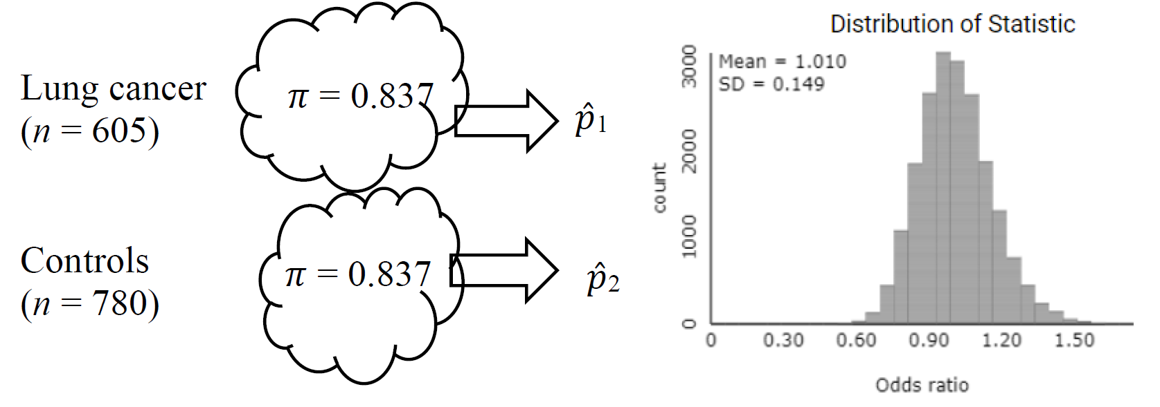
To simulate outcomes for a case-control study, we can treat the numbers of cases (lung cancer patients) and control patients as fixed, and randomly sample from each of these populations, determining the proportion that are "success" (e.g., heavy smokers). Under the null hypothesis, we could use 1159/1385 ≈ 0.837 as the common probability of success in the Comparing Two Population Proportions applet and generate a sampling distribution of odds ratios.
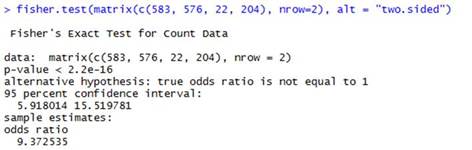
The null distribution of odds ratios has a mean around 1, and set up this way, the observed odds ratio of 9.385 produces a very small p-value. (This p-value is equivalent to the Fisher’s Exact Test p-value.)
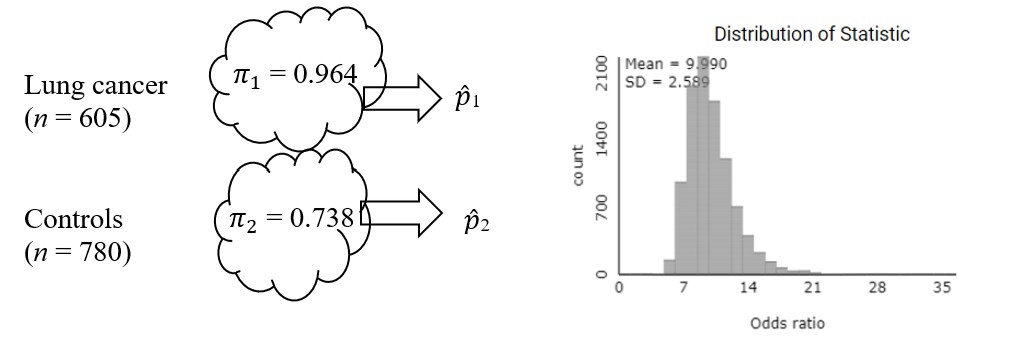
To estimate a confidence interval, we could instead use the sample proportions (583/605 and 576/780) as the process probabilities, rather than assuming they are equal.
The center of this distribution is now around 10, similar to the observed odds ratio, and the standard deviation is around 2.6. We also notice these distributions are slightly skewed to the right. We can again use a log-transformation to see whether that creates a more symmetric distribution as was the case for relative risk.
Keep in mind that this distribution does not assume the null hypothesis is true, so we shouldn’t use this distribution to find a p-value directly. But we are very interested in the variability of this distribution.
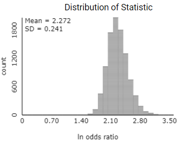
The sampling distribution of the sample odds ratio also follows a log-normal distribution like the relative risk. Thus, we can construct a confidence interval for the population log-odds ratio using the normal distribution. The standard error of the sample log-odds ratio (using the natural log) is given by the expression:
8.Calculate Standard Error and Confidence Interval.
Calculate this standard error (and compare to the simulation results) and then use it (by hand) to find an approximate 95% confidence interval for the log odds ratio.
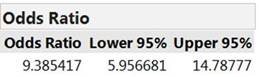
We are 95% confident that the heavy smokers’ odds of being a lung cancer patient rather than a control patient are 5.96 to 14.79 times higher than the odds for a light smoker being a lung cancer patient rather than a control patient. (This is the alternative interpretation of the value of tau defined in g.)
This interval does not contain one, matching our small p-value. Both the test and confidence interval say it is not plausible that the odds of lung cancer are the same for both heavy and light smokers.
Summarize (with justification) the conclusions you would draw from this study (using both the p-value and the confidence interval, and addressing both the population to which you are willing to generalize and whether or not you are drawing a cause-and-effect conclusion).
This study gives us strong evidence that the odds of being a lung cancer patient are quite a bit larger for those who are regular to heavy smokers compared to the lighter or non-smokers. We can’t attribute this increase to the smoking habit alone because this was an observational (case-control) study rather than a randomized experiment, though they did match age and economic factors between the two groups. But there could be other differences like in diet and exercise that account for the higher rate of lung cancer among the heavy smokers. We also should be a little cautious in generalizing these results, perhaps only to hospitalized males like those selected by these researchers (age, social-economic status).
Because the baseline incidence of lung cancer in the population is so small, the researchers conducted a case-control study to ensure they would have both patients with and without lung cancer in their study (matched by age and economic status). In a case-control study, the odds ratio is a more meaningful statistic to compare the incidence of lung cancer between the two groups. We find that the sample odds of lung cancer are almost ten times larger for the regular smokers compared to the non-regulars in this study. By the invariance of the odds ratio, this also tells us that the odds of being a regular smoker (rather than not) are almost 10 times higher for those with lung cancer. We are 95% confident that in the larger populations represented by these samples, the odds of lung cancer are 5.92 to 15.52 times larger for the regular smokers (Fisher’s Exact Test p-value ≪ 0.001). If both success proportions had been small, we could say this is approximately equal to the relative risk and use the words "10 times higher" or "10 times more likely." The full data set (which broke down the second category further) also shows that the odds of having lung cancer increase with the amount of smoking (light smokers have 2 times the odds, heavy smokers have 11 times the odds, and chain smokers have 29 times the odds!)—this is called a "dose-response." We see a strong relationship between the size of the "dose" of smoking and occurrence of lung cancer for these patients.
However, this study was criticized for "retrospective bias" in asking subjects to accurately remember, and be willing to tell, details of their lifestyles. This can also be complicated by asking these questions of patients who know they have been diagnosed with lung cancer, as their recall may be affected by this knowledge. We also have to worry whether hospitalized males are representative of the general male population. Other studies around the same time (e.g., Hammond and Horn – see Practice Problem 3.10, Wynder and Cornfield) found similar increases in "risk" with smoking. However, these were all observational studies so critics reasonably argued that other variables such as lifestyle, diet, exercise, and genetics could be responsible for both the smoking habits and the development of lung cancer. Although there was still much (on-going) research to be done, and these studies did not claim to prove that cigarette smoking causes lung cancer, these landmark studies set the stage. They also led to many efforts in improving study design and in developing statistical tools (such as relative risk and odds ratios) to analyze the results.
A researcher searched court records to find 908 individuals who had been victims of abuse as children (11 years or younger). She then found 667 individuals, with similar demographic characteristics, who had not been abused as children. Based on a search through subsequent years of court records, she determined how many in each of these groups became involved in violent crimes (Widom, 1989). The results are shown below:
Create a sampling distribution for the odds ratio [Hint: Which variable was "controlled" by the researcher? What is your estimated common probability of success?]
Create a sampling distribution for the log-odds ratio. Does the normal approximation appear appropriate? Report the mean and standard deviation of this distribution.
Report the p-value from Fisher’s Exact Test. Which of the previous p-values is this closest to? Why? Do the p-values vary much? Which would you consider the "best"? Why?
Is it reasonable to conclude that being a victim of abuse as a child causes individuals to be more likely to be violent toward others afterwards? Explain.
Suppose that individuals in Group 1 have a 2/3 probability of success, and those in Group 2 have a 1/2 probability of success. Calculate and interpret the relative risk of success, comparing Group 1 to Group 2.