Investigation 3.8: Peanut Allergies

Section 12.4 Investigation 3.8: Peanut Allergies

Peanut allergies have increased in prevalence in the last decade, but can they be prevented? Even among infants with a high risk of allergy? Is it better to avoid the problematic food or to encourage early introduction?

🔗

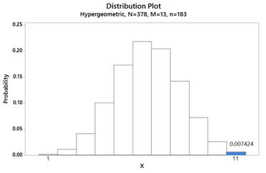
Du Toit et al. (New England Journal of Medicine, Feb. 2015) randomly assigned U.K. infants (4-11 months old) with pre-existing sensitivity to peanut extract to either consume 6 g of peanut protein per week or to avoid peanuts until 60 months of age. The table below shows the results for infants who were not initially sensitized to peanuts and whether or not the child had developed a peanut allergy at 60 months.

🔗

Table 12.4.1.

🔗

	Peanut avoidance	Peanut consumption	Total
Peanut allergy	11	2	13
No allergy	172	193	365
Total	183	195	378

Checkpoint 12.4.2. Calculate Proportions.

Calculate the proportion of children who developed a peanut allergy. Then calculate the proportion of children developing a peanut allergy in each group. Does this appear to be a large difference to you?

🔗

Solution.

Overall: 13/378 = 0.034 or 3.4%

🔗

Avoidance: 11/183 = 0.060 or 6.0%

🔗

Consumption: 2/195 = 0.010 or 1.0%

🔗

The difference is 5 percentage points, which may not seem large numerically but represents a 6-fold difference.

🔗

Aside: Two-way Table Applet.

Checkpoint 12.4.3. Fisher’s Exact Test.

Use Fisher’s Exact Test to investigate whether these data provide convincing evidence that the probability of developing a peanut allergy is larger among children who avoid peanuts for the first 60 months. Do you consider this strong evidence that the peanut consumption effectively deters development of a peanut allergy in this population?

🔗

Hint.

State the hypotheses in symbols and in words. Define the random variable and outcomes of interest in computing your p-value.

🔗

Solution.

H0: πavoid = πconsume (no difference in allergy probability)

🔗

Ha: πavoid > πconsume (higher allergy probability with avoidance)

🔗

Let X = number with peanut allergy in avoidance group. p-value = P(X ≥ 11) where X ~ Hypergeometric(N=378, M=13, n=183)

🔗

p-value ≈ 0.0074, which provides strong evidence that avoiding peanuts increases the probability of developing an allergy.

🔗

Checkpoint 12.4.4. Comparing Proportions.

Would you feel any differently about the magnitude of the difference in proportions if the conditional proportions developing a peanut allergy had been 0.500 and 0.55? Explain.

🔗

Solution.

Yes, a difference of 0.05 (5 percentage points) seems much less impressive when the base rates are 50% and 55% compared to 1% and 6%. The absolute difference is the same, but the relative change is quite different.

🔗

Discussion.

When the baseline rate (probability) of success is small, an alternative statistic to consider rather than the difference in the conditional proportions (which will also have to be small by the nature of the data) is the ratio of the conditional proportions. First used with medical studies where "success" is often defined to be an unpleasant event (e.g., death), this ratio was termed the relative risk.

🔗

Definition: Relative Risk.

The relative risk is the ratio of the conditional proportions, often intentionally set up so that the value is larger than one:

🔗

\begin{equation*} RR = \frac{\hat{p}_1}{\hat{p}_2} \end{equation*}

🔗

where \(\hat{p}_1\) is the larger proportion and \(\hat{p}_2\) is the smaller proportion.

🔗

The relative risk tells us how many times higher the "risk" or "likelihood" of "success" is in group 1 compared to group 2.

🔗

Checkpoint 12.4.5. Calculate Relative Risk.

Determine and interpret the ratio of the conditional proportions who developed peanut allergy between the peanut avoiders and the peanut consumers in this study.

🔗

Solution.

Relative risk = 0.060 / 0.010 = 5.85

🔗

Children who avoided peanuts were about 5.85 times more likely to develop a peanut allergy than children who consumed peanuts.

🔗

Checkpoint 12.4.6. Percentage Change.

Because we are now working with a ratio, we can also interpret this statistic in terms of percentage change. Subtract one from the relative risk value and multiply by 100% to determine what percentage higher the proportion who developed a peanut allergy is in the avoidance group compared to the consumption group.

🔗

Solution.

(5.85 - 1) × 100% = 485%

🔗

The proportion who developed a peanut allergy is 485% higher in the avoidance group.

🔗

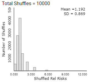
Of course, now we would also like a confidence interval for the corresponding parameter, the ratio of the underlying probabilities of allergy between these two treatments. When we produced confidence intervals for other parameters, we examined the sampling distribution of the corresponding statistic to see how values of that statistic varied under repeated random sampling. So now let’s examine the behavior of the relative risk of conditional proportions using the Analyzing Two-Way Tables applet to simulate the random assignment process (as opposed to simulating the random sampling from a binomial process) under the (null) assumption that there’s no difference between the two treatments. [See the Technology Detour below for software instructions.]

🔗

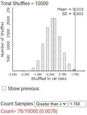
Checkpoint 12.4.7. Generate Null Distribution.

Generate a null distribution for Relative Risks:

🔗

Check the 2×2 box

🔗
Enter the two-way table into the applet and press Use Table.

🔗
Generate 10,000 random shuffles.

🔗
Use the Statistic pull-down menu to select Relative Risk.

🔗

🔗

Describe the behavior of the null distribution of relative risk values.

🔗

Solution.

The distribution should be centered around 1 (no difference) and skewed to the right.

🔗

Example results

🔗

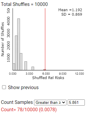
Checkpoint 12.4.8. Observed Value in Null Distribution.

Where does the observed value of the relative risk from the actual study fall in the null distribution of the relative risks? What proportion of the simulated relative risks are at least this extreme?

🔗

Solution.

The observed value (5.85) should be far out in the right tail. Very few (less than 1%) of the simulated values should be this extreme or more.

🔗

But can we apply a mathematical model to this distribution?

🔗

Checkpoint 12.4.9. Mean Near 1.

Why does it make sense that the mean of the simulated relative risks is close to the value 1?

🔗

Hint.

Remember the assumption behind your simulation analysis.

🔗

Solution.

Under the null hypothesis, the two treatments are equally effective, so the ratio of the probabilities should be 1 (no difference).

🔗

Checkpoint 12.4.10. Skewness.

You should notice skewness in the distribution of relative risk values. Explain why it is not surprising for the distribution of this statistic to be skewed to the right (especially with smaller sample sizes).

🔗

Solution.

A ratio can be any positive value. Values close to 1 are restricted to fall between 0 and 2, but large ratios can extend far to the right (e.g., 5, 10, 100, etc.). This creates right skewness.

🔗

Note: If the number of successes in either group equals zero, the applet adds 0.5 to each cell of the table before calculating the relative risk in order to avoid dividing by zero.

🔗

In fact, this distribution is usually well modeled by a log normal distribution.

🔗

Checkpoint 12.4.11. Log Transformation.

To verify this, check the ln relative risk box (in the lower left corner, or choose from pull-down menu) to take the natural log of each relative risk value and display a new histogram of these transformed values. Describe the shape of this distribution. Is the distribution of the lnrelrisk well modeled by a normal distribution?

🔗

Solution.

After taking the natural log, the distribution should be approximately symmetric and bell-shaped (normal).

🔗

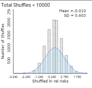
Checkpoint 12.4.12. Mean of Log Relative Risk.

What is the mean of the simulated lnrelrisk values? Why does this value make sense?

🔗

Solution.

The mean should be close to 0, which makes sense because ln(1) = 0.

🔗

Checkpoint 12.4.13. Standard Deviation.

What is the standard deviation of the lnrelrisk values?

🔗

Solution.

Results will vary but should be around 0.8-1.0.

🔗

Checkpoint 12.4.14. Observed Log Relative Risk.

Calculate the observed value of \(ln(\hat{p}_1/\hat{p}_2)\) for this study (but don’t round up). Where does this value fall (near in the middle or in the tail) of this simulated distribution of lnrelrisk values? Find the empirical p-value by counting the number of lnrelrisk values at least as extreme.

🔗

Solution.

ln(5.85) = 1.767. This should fall far in the right tail of the distribution, with a p-value around 0.007-0.008.

🔗

Checkpoint 12.4.15. Change in p-value?

Has the empirical p-value changed? Explain why this makes sense.

🔗

Hint.

What does change about the distribution when you take the natural log of every value?

🔗

Solution.

No, the p-value has not changed. Taking the log is a monotonic transformation, so it doesn’t change the ranking of values or which ones are extreme.

🔗

While the log transformation does not impact the p-value, it does impact the confidence interval. So far you have seen the standard deviation of the null distribution, but that assumes the probability of success is the same for both treatments. Instead, we want to find a standard deviation of the ln rel risk values without making that assumption.

🔗

Theoretical Result.

It can be shown that the standard error of the ln relative risk is approximated by:

🔗

\begin{equation*} SE(\ln(RR)) = \sqrt{\left(\frac{1}{A} - \frac{1}{A+B}\right) + \left(\frac{1}{C} - \frac{1}{C+D}\right)} \end{equation*}

🔗

where \(A\text{,}\) \(B\text{,}\) \(C\text{,}\) and \(D\) are the observed counts in the 2×2 table of data, with \(A\) and \(C\) representing the number of "successes" in the two groups. Having this formula allows us to determine the variability from sample to sample without conducting the simulation first.

🔗

Checkpoint 12.4.16. Calculate Standard Error.

Calculate the value of this standard error of the ln(rel risk) for this study. Interpret this value and compare it to the standard deviation from your simulated lnrelrisk values.

🔗

Solution.

\begin{equation*} SE = \sqrt{\left(\frac{1}{11} - \frac{1}{183}\right) + \left(\frac{1}{2} - \frac{1}{195}\right)} \end{equation*}

\begin{equation*} = \sqrt{0.0854 + 0.4949} = \sqrt{0.5803} = 0.762 \end{equation*}

This should be reasonably close to (but somewhat different from) the simulation SD, as we’re not assuming the null hypothesis is true.

🔗

Note: The variability in the statistic under the null hypothesis (as estimated by the simulation) should be in the ballpark but not all that close to the variability in the statistic estimated from the data. If we used a pooled \(\hat{p}\text{,}\) modelling the null hypothesis to be true, the results are usually a bit more similar: Assuming null hypothesis is true: \(\sqrt{1/6.34 - 1/183 + 1/6.76 - 1/195} \approx 0.543\text{.}\) In a case like this where we have strong evidence against the null hypothesis, using the observed counts is more appropriate.

🔗

Checkpoint 12.4.17. Confidence Interval Formula.

Now that you have a statistic (ln rel risk) that has a sampling distribution that is approximately normal and you have a value for the standard deviation of the statistic from checkpoint 15, what general formula can we use to determine a confidence interval for the parameter?

🔗

Solution.

statistic ± (critical value) × SE

🔗

For 95% CI: ln(rel risk) ± 1.96 × SE(ln rel risk)

🔗

Checkpoint 12.4.18. Calculate Confidence Interval.

Calculate the midpoint, 95% margin-of-error, and 95% confidence interval endpoints using the observed value of ln(rel risk) as the statistic and using the standard error calculated in checkpoint 15.

🔗

Solution.

Midpoint: ln(5.85) = 1.767

🔗

Margin of error: 1.96 × 0.762 = 1.494

🔗

95% CI: (1.767 - 1.494, 1.767 + 1.494) = (0.273, 3.261)

🔗

Checkpoint 12.4.19. Parameter Estimated.

What parameter does the confidence interval in checkpoint 18 estimate?

🔗

Solution.

ln(πavoid / πconsume), the natural log of the relative risk

🔗

Checkpoint 12.4.20. Exponentiate Endpoints.

Exponentiate the endpoints of this interval to obtain a confidence interval for the ratio of the probabilities of developing a peanut allergy between these two treatments. Interpret this interval.

🔗

Solution.

95% CI for relative risk: \((e^{0.273}, e^{3.261}) = (1.31, 26.08)\)

🔗

We are 95% confident that children who avoid peanuts are between 1.31 and 26.08 times more likely to develop a peanut allergy than children who consume peanuts.

🔗

Checkpoint 12.4.21. Zero in Interval?

Is zero in this interval? Do we care? What value is of interest instead?

🔗

Solution.

No, zero is not in the interval, but that’s not relevant. For relative risk, the value of interest is 1 (no difference). Because 1 is not in the interval, we have evidence of a difference.

🔗

Checkpoint 12.4.22. Midpoint of CI.

Is the midpoint of this confidence interval for the population relative risk equal to the observed value of the sample relative risk? Explain why this makes sense.

🔗

Solution.

No, the midpoint is \(e^{1.767} = 5.85\text{,}\) which equals the observed relative risk. But the interval (1.31, 26.08) is not symmetric around 5.85 because we’re working on the log scale and then exponentiating back.

🔗

Checkpoint 12.4.23. Compare to Applet.

Compare the confidence interval you just calculated to the one given by the applet if you now check the 95% CI for relative risk box. Note: The confidence interval for the relative risk will not necessarily be symmetric around the statistic.

🔗

Solution.

The intervals should match closely.

🔗

Checkpoint 12.4.24. Coverage Probability.

Suppose you used this method to construct a confidence interval for each of the 1,000 simulated random samples that you generated in checkpoint 7. Because our simulation assumes the null hypothesis to be true, do you expect the value 1 to be in these intervals? All of them? Most of them? What percentage of them? Explain.

🔗

Solution.

We would expect about 95% of the intervals to contain the value 1, because under the null hypothesis, the true relative risk is 1, and we’re using 95% confidence intervals.

🔗

Study Conclusions.

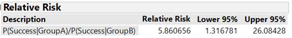
This study provided strong evidence that children with pre-existing sensitivity to peanut extract are more likely to develop a peanut allergy by 5 years of age if they avoid consuming peanuts than if they consume peanuts (exact one-sided p-value = 0.0074, z-score = 2.66). To estimate the size of the difference, focusing on the difference in "success" probabilities has some limitations. In particular, if the probabilities are small it may be difficult for us to interpret the magnitude of the difference between the values. Also, we have to be very careful with our language, focusing on the difference in the allergy probabilities and not the percentage change. An alternative is to construct a confidence interval for the relative risk (ratio of conditional probabilities). An approximation exists (even with rather small sample sizes) for a z-interval for the ln(relative risk) which can then be back-transformed to an interval for long-run relative risk. Many practitioners prefer focusing on this ratio parameter rather than the difference. From this study, we are 95% confident that ratio of the probabilities of peanut allergy is between 1.32 and 26.08. This means that avoiding peanuts rather than consuming some 6g/week raises the probability of developing a peanut allergy by between 32% and 2500%.

🔗

Note: It can be risky to interpret the relative risk in isolation without considering the absolute risks (conditional proportions) as well. For example, doubling a very small probability may not be noteworthy, depending on the context. You should also note that the percentage change calculation and interpretation depends on which group (e.g., treatment or control) is used as the reference group.

🔗

Note: Efficacy is defined as 1 – risk of vaccinated group/risk of unvaccinated group × 100%.

🔗

Subsection 12.4.1 Practice Problem 3.8A

Checkpoint 12.4.25. Confidence Interval for No Allergy.

For the peanut allergy study, find a 95% confidence interval for the probability of not developing a peanut allergy comparing the consumption treatment to the avoidance treatment.

🔗

Checkpoint 12.4.26. Interpret Interval.

Provide a one-sentence interpretation of the interval in the previous checkpoint.

🔗

Checkpoint 12.4.27. Compare Intervals.

Is the interval the same or closely related to the one you found in Investigation 3.8? Does one interval provide strong evidence of a treatment effect? Which interval would you report to new parents?

🔗

Checkpoint 12.4.28. Statistical Power.

The article reports that "the power to detect a difference in risk of 30 percentage points was 80.0%." Explain what this means in your own words.

🔗

Subsection 12.4.2 Practice Problem 3.8B: Knee Surgery Study

A multicenter, randomized, double-blind trial involved patients aged 36-65 years who had knee injuries consistent with a degenerative medial meniscus tear (Shivonen et al., New England Journal of Medicine, 2013). Patients received either the most common orthopedic procedure (arthroscopic partial meniscectomy, \(n_1 = 70\)) or sham surgery that simulated the sounds, sensations, and timing of the real surgery (\(n_2 = 76\)). After 12 months, 54 of those in the treatment group reported satisfaction, compared to 53 in the sham surgery.

🔗

Checkpoint 12.4.29. Relative Risk CI.

Calculate and interpret a confidence interval for the ratio of the probabilities (relative risk) of satisfaction for these two procedures.

🔗

Checkpoint 12.4.30. Interpretation.

What does your interval in the previous checkpoint indicate about whether those receiving the orthopedic surgery are significantly more likely that those receiving a sham surgery to report satisfaction after 12 months? Explain your reasoning.

🔗

You have attempted of activities on this page.

🔗

Prev Top Next