Exercises 5.2.1 Background
The authorship of literary works is often a topic for debate. Were some of the works attributed to Shakespeare actually written by Bacon or Marlowe? Which of the anonymously published Federalist Papers were written by Hamilton, which by Madison, which by Jay? Who were the authors of the writings contained in the Bible? The fields of "literary computing" and "forensic stylometry" examine ways of numerically analyzing authors’ works, looking at variables such as sentence length and rates of occurrence of specific words.
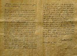
The passage you selected words from is Abraham Lincoln’s Gettysburg Address, given November 19, 1863 on the battlefield near Gettysburg, PA. In characterizing this passage, we would ideally examine every word. However, often it is much more convenient and even more efficient to only examine a subset of words.
Definitions: Population, Sample, and Sample Size.
The
population is the entire collection of observational units that we are interested in. A
sample is the subset of the population for which we collect data. A study’s
sample size is the number of observational units in the study.
In this investigation you will examine data for just 10 of the 268 words in the Gettysburg Address. We are considering this passage to be a population of 268 words, and the 10 words you selected are therefore a sample from this population. Now we define the sample as a collection of individuals or observational units that have distinct characteristics, rather than a finite set of repeated realizations of a random process.
In most statistical studies, we do not have access to the entire population and can consider only data for a sample from that population. Our ultimate goal is to make (appropriate) conclusions about the larger population, based on only the sample data.
Up until now, we have generally been assuming we have a representative sample from an infinite on-going process (e.g., toast drops, hospital transplant operations, candy manufacturing). We made some assumptions, like the process is not changing over time and that there is no tendency to select some types of outcomes more than others (e.g., getting the first 5 candies from the manufacturing process rather than throughout the day). In fact, a binomial process assumes you have repeat observations from the exact same process but with randomness in the actual outcome that occurs (sometimes an infant chooses the helper toy, sometimes not; the randomness is in the choice).
In this investigation, instead of sampling from an on-going process we are sampling from a finite population (the 268 words). In fact, we actually have access to the entire population. But what if we didn’t? We still need some way of convincing people that our sample is likely to be representative of the population. Let’s use this population to explore how samples behave when the "random chance" arises from which observational units are selected to be in the sample, rather than from "random choices" made by the observational units.
1. Your sample of words.
Paste your 10 words from the data collection activity below. This will help you reference them as you work through the investigation.
Tip: You will use these words to answer the questions below.
2. Calculating sample proportion of short words.
Looking at your 10 words, define "short" to be 3 or fewer letters. Determine how many of your 10 words are short and calculate the proportion of short words in your sample.
Hint.
Count the number of words with 3 or fewer letters, then divide by 10.
3. Identifying observational units and variables.
Identify the observational units (objects being studied) and variable for this sample.
Hint.
What are the individual entities being measured? What characteristic are we recording about each one?
Solution.
Observational units: words
Variable: Is the word short or long?
4. Variable type.
What type of variable is this?
Solution.
Type: (binary) categorical
Definitions: Parameter and Statistic.
The term
parameter, before considered the process probability, is also used to refer to a numerical characteristic of a population. We will continue to denote population parameters with Greek letters, for example
\(\pi\) or
\(\mu\) for a population proportion or population mean, respectively.
A
statistic continues to be the corresponding number but calculated from sample data. We denote the statistics for a sample proportion and a sample mean by
\(\hat{p}\) and
\(\bar{x}\text{,}\) respectively.
5. Sample statistic vs. population parameter.
Is the proportion of short words you calculated in
Question 2 a parameter or a statistic?
Hint.
Were you calculating from a sample or from the entire population?
Solution.
Statistic, calculated from a sample of ten words,
\(\hat{p}\text{.}\) This is the value we observe from our sample.
6. Symbol.
What symbol should we use for the proportion of short words you calculated in
Question 2?
-
\(\pi\)
-
-
\(\mu\)
-
-
\(\hat{p}\)
-
-
\(\bar{x}\)
-
7. Identifying the population parameter.
The proportion of all 268 words in this population that are short is 0.41. Is this number a parameter or a statistic?
Hint.
This proportion is calculated from all 268 words, not just a sample.
Solution.
Parameter,
\(\pi\text{.}\)
8. Symbol.
What symbol should we use to represent the proportion of all 268 words in this population that are short?
-
\(\pi\)
-
-
\(\mu\)
-
-
\(\hat{p}\)
-
-
\(\bar{x}\)
-
9. Sampling variability.
Did everyone in your class obtain the same sample proportion?
Hint.
Think about what the distribution of many sample proportions would look like if the method is unbiased.
Solution.
Answers will vary but no student’s sample proportion could be 0.41 exactly, and it is unlikely that everyone obtained the same sample proportion. To decide whether this sampling method tends to produce samples that are representative we could plot the sample averages and compare the center of the distribution to 0.41.
10. Describing representative sampling.
Describe a way for deciding whether this sampling method tends to produce samples that are representative of the larger population for this parameter.
11. Creating a dotplot of class results.
To view a dotplot of your class’s sample proportions, enter your class section identifier below to generate a custom URL.
What does each dot in this dotplot represent?
Hint.
What would have to be done to add another dot to the graph?
Solution.
Each dot in the dotplot represents the sample proportion of short words from one student’s sample of 10 words. Since each student selected a different sample of 10 words, each calculated a different sample proportion, which appears as a separate dot in the distribution.
12. Interpreting the sampling distribution.
What does the graph in
Question 11 tell you about whether this sampling method tends to produce representative samples?
Hint.
Look at where the center of the distribution is. Is it close to the population proportion of 0.41?
Solution.
Example results. Each dot in the graph represents the proportion of short words in a random sample of 10 words.
sols.jpg)
Solution graph showing sampling distribution - Mean = 0.2019, SD = 0.1704, median = 0.20, \(n\) = 53
Mean = 0.2019, SD = 0.1704, median = 0.20,
\(n\) = 53.
Discussion.
You have again witnessed the fundamental principle of
sampling variability: Values of sample statistics vary when one takes different samples from the same population. The distribution of statistics from a repeated sampling is often called a
sampling distribution. In this case, we are treating each sample as an observational unit and the sample statistics as the variable of interest (so the graph label should be something like "sample proportion short"). Although we clearly expect there to be sample-to-sample variation in the statistic, there is a problem if there is a tendency to over- or under-estimate the parameter of interest.
Definition: Bias and Unbiased Sampling.
When characteristics of the resulting samples are systematically different from characteristics of the population, we say that the sampling method is
biased. When the distribution of the sample statistics, under repeated sampling from the same population, is centered at the value of the population parameter, the sampling method is said to be
unbiased.
For example, we suspect that your class repeatedly and consistently underestimated the proportion of short words. Not everyone has to underestimate, but if there is a tendency to err in the same direction time and time again, then the sampling method is biased. In other words, sampling bias is evident if we repeatedly draw samples from the population and the distribution of the sample statistics is not centered at the population parameter of interest. Note that bias is a property of a sampling method, not of a single sample. Studies have shown that human judgment or "convenience sampling" (e.g., selecting the most readily available observational units) is not a good basis for selecting representative samples, so we will rely on other techniques to do the sampling for us.
13. Direction of bias.
Do your class results indicate a tendency to overestimate or to underestimate the population proportion
\(\pi\text{?}\)
Hint.
Think about what types of words people tend to notice or select when choosing "representative" words.
-
Overestimate
-
-
Underestimate
-
Solution.
Because most of the sample proportions are less than 0.41, this sampling method tends to under-estimate the population proportion and is therefore not representative.
The class results indicate a tendency to underestimate
\(\pi\) = 0.41. This could have been predicted in advance - we all tend to select longer words because we tend to overlook short words like "a", "the" and "of".
14. Predicting bias.
Could you have predicted that in advance? Explain.
Solution.
Yes. When people are asked to select representative words, they tend to overlook short words like "a", "the" and "of", and instead select longer, more interesting words. Therefore, this sampling method tends to under-estimate the proportion of short words in the Gettysburg Address.
15. Alternative sampling method.
Consider another sampling method: you close your eyes, point at the passage of words, select whatever word your pen lands on, and repeat this 10 times. Would this sampling method be biased?
Hint.
Think about whether longer words are easier to point at than shorter words.
Solution.
This sampling method would also be biased - longer words take up more space on the page and are therefore more likely to be "hit" by your pen. This sampling method would also tend to under-estimate the proportion of short words in the Gettysburg Address.
Taking samples of 20 words would have no effect on the bias of this sampling method. We would just end up with samples of 20 long words.
16. Direction of bias in alternative method.
If so, in which direction?
-
Overestimate
-
-
Underestimate
-
-
Not biased
-
17. Effect of sample size on bias.
What if you looked at 20 words instead of 10? Would you expect this sampling method to still be biased?
-
Yes, still biased
-
-
No, not biased
-
-
Not sure
-
18. Suggest a better method.
Suggest a better method for selecting a sample of 10 words from this population that is likely to be representative of the population.
Hint.
What sampling method would give every word an equal chance of being selected?
Solution.
Randomly! Use a random selection method such as assigning each word a number and using a random number generator to select which words to include in the sample. This gives every word an equal chance of being selected, regardless of its length or position.
Definition: Simple Random Sample.
A
simple random sample gives every observational unit in the population the same chance of being selected. In fact, it gives every sample of size n the same chance of being selected.
So, with a simple random sample of size 10, any set of 10 words is equally likely to end up as our sample.
The first step is to obtain a list of every member of your population (this list is called a
sampling frame). Then, give each observational unit on the list a unique ID number.
You can view the
numbered sampling frame for the passage, with each word in the population numbered. You can use technology to select a 3-digit number at random, and then match it to the word in the population with that ID number. Then repeat to randomly select additional (unique) IDs (words).
Technology Detour – Selecting a Simple Random Sample.
19. Technology Detour (Applet).
You may use
random.org or our Generate Random Numbers applet to select a simple random sample of integers by specifying the range of integers (e.g., 1 to 268) and, if an option, how many numbers you want to generate.
Hint.
To generate 5 random numbers between 1 and 268, specify those values in the random number generator.
20. Other options.
Or use R or JMP to select a simple random sample of 5 ID numbers from 1 to 268. Click on the hint below for instructions.
Hint 1. R/Sage Instructions
Create a list of integers from 1 to 268 and take a simple random sample of 5 ID numbers. Click "Evaluate (R)" to generate your sample. You can click "Evaluate" multiple times to get different samples.
Hint 2. JMP Instructions
To select a simple random sample in JMP:
-
Choose
File > New > Data Table.
-
From the
Rows menu, select
Add Rows. Add 5 rows to the table. Press
OK.
-
Right click the column heading. Select
Formula.
-
Under
Random select
Random Integer.
-
Enter 1 and 268 as the bounds. Click
OK.
Note: The Random Integer function will generate random integers within the specified range for each row in your data table.
Solution.
Each time you run
sample(ids, 5), you will get 5 different random numbers between 1 and 268. Example output: 45, 162, 3, 210, 97
-
Several variables on the words in the Gettysburg Address have already been preloaded. Use the
Choose variable pull-down menu to change the variable to
Short. Verify our claim about the value of the population proportion.
-
Check the
Show Sampling Options box. Specify 5 as the
Sample size. Press
Draw Samples.
21. Sample proportion from random sample.
How many of the words selected by the computer were short? Confirm the computer’s calculation of the sample proportion and report below.
22. Comparing distributions.
Combine your results with your classmates to produce a dotplot of the proportions of short words. Comment on the distribution and particularly how it compares to the one in
Question 11.
Solution.
Mean = 0.494, SD = 0.53294, median = 0.40,
\(n\) = 53. This graph is centered much closer to 0.41, with a standard deviation that is about half as large.
23. Sampling variability with random samples.
When taking random samples, did everyone obtain a sample proportion equal to the population proportion or is there still sample to sample variation?
Solution.
No one obtained a sample proportion equal to the population proportion (it is impossible to obtain a sample proportion of 0.41 when
\(n\) = 5), but there was definitely sample to sample variation. Not everyone got the same sample proportion of short words.
24. Better sample results.
So then in what way would you say these random samples produce "better" sample results than the "circle 10 words" method?
Solution.
Even with the smaller sample size, the improved selection method reduced the bias - these sample proportions did not tend to under- (or over-) estimate
\(\pi\text{.}\)
Of course, to really see the long-term pattern of the sampling distribution of the statistic, we would like to take many more random samples from this population.
In the Sampling Words applet,
-
Change the
Number of Samples from 1 to 999 (for 1,000 total)
-
25. Behavior of sampling distribution.
Describe the behavior of the distribution of sample proportions. Would you say the computer is using an unbiased sampling method? How are you deciding?
Hint.
Look at where the distribution is centered. Is it close to the population proportion of 0.41? Is the distribution systematically over or under that value?
Solution.
The distribution is fairly symmetric and centered close to 0.41. The computer appears to be using an unbiased sampling method because the sample proportions are not systematically over or under 0.41.
26. Comparing sampling methods.
Notice that you took a smaller sample (
\(n\) = 5) with the applet than when you circled the words (
\(n\) = 10). Which sampling method was less biased?
Solution.
The computer’s sampling (simple random samples) method appears less biased.
27. Prediction for larger sample size.
Prediction: Suppose we use the computer to take samples of size 10 instead, how do you predict the distribution of sample proportions will change?
28. Testing the prediction.
How/Has the distribution changed? Is this what you predicted?
Solution.
The center has not changed (0.40), nor has the symmetric shape. But the standard deviation has decreased to 0.154.
Discussion.
Even with randomly drawn samples, sampling variability still exists (random sampling errors). Although not every random sample produces the same characteristics as the population, random sampling has the property that the sample statistics do not consistently overestimate the value of the parameter or consistently underestimate the value of the parameter (which is not changing). The means of the above distributions of sample proportions (the statistics) are both very close to 0.41, the population proportion (the parameter). Because the distributions of the sample statistic (as a random variable) are centered at the value of the population parameter, both graphs are considered to demonstrate an unbiased sampling method. With random samples,
\(E(\hat{p}) = \pi\text{,}\) even when sampling from a finite population.
Notice that in judging bias we are concerned only with the mean of the distribution, not the shape or variability. However, if we do take larger samples (
\(n\) = 10 rather than
\(n\) = 5), we improve the precision of our statistics as they will tend to cluster even more tightly around the population proportion. In designing a study, it is critical to first make sure there is no sampling bias (use random sampling), then the sample size (not the number of samples) will determine how close the statistic can be expected to be to the parameter.
Summary.
We have seen two very desirable properties of sample proportions when using random samples from a large population:
-
The distribution of sample proportions centers at the population proportion (so the sampling method is unbiased).
-
The distribution of sample proportions has less sample-to-sample variability when we increase the sample size (producing increased precision).
Simple random samples are not as simple as they sound. They require a complete sampling frame and 100% response rate. This can be quite a challenge, especially if you are interested in individuals throughout the country for example. There are other probability sampling methods that are typically unbiased. See this
discussion for a brief introduction to cluster sampling, multistage sampling, stratified sampling, and systematic sample. These techniques will come up later in the text and can be much more practical to carry out.
sols.jpg)
sols.jpg)
