Section 5.3 Investigation 1.13: Sampling Words (cont.)
In Section 3, we have transitioned from sampling from an infinite process to sampling from a finite population. We discussed randomly selecting the sample from a list of the entire population as a way to convince critics that the sample is likely to be representative of the larger population and therefore, we are willing to generalize results from a randomly selected sample to the larger population.
So now the “random chance” we are modelling is not in an individual outcome (like in a coin flip) but in which individuals we obtain in our sample. As suggested in Investigation 1.12, sample statistics from random samples will again follow a predictable pattern, allowing us to measure the strength of evidence against claims about the population parameter and to estimate the margin-of-error in our estimates of the parameter. We will again consider simulation-based p-values, exact p-values, and a mathematical model for estimating the p-value and confidence interval.
Exercises 5.3.1 Estimating the Standard Deviation of Sample Proportions
In the previous investigation, we saw that if we take random samples from a finite population, the mean of the sampling distribution of sample proportions should equal the population proportion (i.e., \(E(\hat{p}) = \pi\)). But what about the standard deviation of the distribution of sample proportions?
One option is the same formula we used before: \(SD(\hat{p}) = \sqrt{\frac{\pi(1-\pi)}{n}}\text{.}\)
2. Using the Sampling Words Applet.
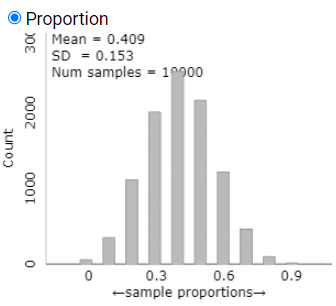
Use the applet below or in a new tab to generate a distribution of 10,000 random samples of size \(n = 10\text{,}\) calculating the sample proportion of words that are short each time.
-
Change the Variable to
Short. -
Check the Show Sampling Options box.
-
Set the Number of Samples to 10000
-
Set the Sample size to 10
-
Press Draw Samples.
3. Simulated standard deviation for \(n\) = 10.
What does the applet report for the standard deviation of the sample proportions? Is it close to the theoretical value you calculated in Question 1?
Applet standard deviation:
Comparison:
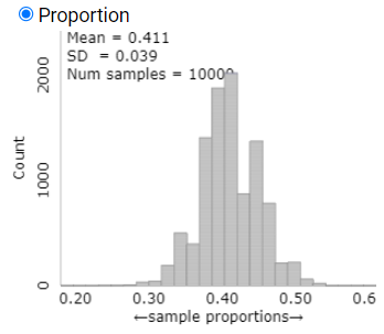
4. Comparing formula and simulation for \(n\) = 100.
Discussion.
The theoretical formula we’ve been using for the standard deviation of sample proportions assumes that the probability of success is constant and the trials are independent (properties of a binomial random variable). Now that we are sampling without replacement from a finite population, the population characteristics do change slightly as we remove observations. The probability the first word is short will be \(110/268 \approx 0.410\text{,}\) but if that word is short, the probability the next one will also be short is now \(109/267 \approx 0.408\text{.}\) And if the first word is not short, the probability the second one will be is \(110/267 \approx 0.412\text{.}\) In other words, the probability of success (short word) for the second trial depends on what we obtained in the first trial.
Key Result: Sampling Without Replacement.
When sampling without replacement from a finite population, the observations are not independent.
This means we can no longer use the binomial distribution to calculate a theoretical standard deviation. This impacts our p-value calculations and our confidence intervals. In particular, the predicted standard deviation is too large, and our confidence intervals will have higher coverage rates than we need.
However, we can use a slightly different formula that corrects for the lack of independence. (The explanation for this formula is in Investigation 1.15.)
Definition: Finite Population Correction Factor.
Using the finite population correction factor, a better estimate of the sample-to-sample variation in sample proportions is
\begin{equation*}
SD(\hat{p}) = \sqrt{\frac{N-n}{N-1}} \cdot \sqrt{\frac{\pi(1-\pi)}{n}}
\end{equation*}
5. Using the finite population correction.
Compute this formula for the samples of size \(n = 100\text{.}\) How does the prediction of the standard deviation change? Why? How does it compare to the standard deviation of the sample proportions simulated by the applet?
Corrected prediction:
Comparison:
Solution.
\begin{align*}
SD(\hat{p}) \amp= \sqrt{\frac{268-100}{268-1}} \cdot \sqrt{\frac{0.41(0.59)}{100}} = \sqrt{\frac{168}{267}} \cdot 0.049\\
\amp\approx 0.791 \cdot 0.049 \approx 0.039
\end{align*}
The finite population correction factor decreases the predicted value of the standard deviation (always multiplying by a value less than one) and gives a value that is closer to the simulation results.
Discussion.
The finite population correction factor should decrease the predicted value of the standard deviation (always multiplying by a value less than one) and give a value that is closer to the simulation results.
Suppose we have a very large population, how does this impact our calculation of the standard deviation of the sample proportions?
-
In the applet, change the population size by selecting the x100 button.
6. Population proportion with larger population.
7. Effect of larger population size.
Generate 10,000 samples of size \(n = 100\) from this population. Report the mean and standard deviation from your simulation and comment on how they compare to Question 4.
Mean:
Standard deviation:
Comparison:
Because we are now sampling a much smaller fraction of the population, the original formula provides a reasonable prediction of the sample-to-sample variation in the sample proportions. Note that the correction factor \(\sqrt{\frac{N-n}{N-1}}\) is very close to one when \(N\) is large and so it can be ignored!
Key Result: Large Population Approximation.
When the population size is much larger than the sample size, we can model sampling from a finite population as sampling from an infinite process as before. The population size (\(N\)) is considered much larger than the sample size (\(n\)) if \(N > 20 \times n\text{.}\)
If the population size is not large, we use the "finite population correction factor." Probability sampling methods other than simple random sampling would also require calculating a different standard deviation. You can learn more appropriate techniques in a course on sampling design and methods.
Discussion.
Once again you see the fundamental principle of sampling variability. Fortunately, this variability follows a predictable pattern in the long run. With random sampling, we expect the sample proportion to be "representative" of the population proportion. The second key advantage of random sampling is we now know how to estimate the size of the sample-to-sample variation. Sample proportions that are based on larger samples will tend to fall even closer to the population proportion as there is less variability among the sample proportions. So first, select randomly to avoid bias, and then if we can increase the sample size, this will improve the precision of the sample results. Once we know the precision of the sample results in repeated samples, then we can decide whether any one particular sample result can be considered statistically significant or unlikely to happen by chance – by the random sampling process – alone. A small p-value does not guarantee that the sample result did not happen just by chance, but it does allow you to measure how unlikely such a result is.
In Investigation 1.15, you will consider a method for computing an "exact" p-value, taking the population size into account. However, in many situations we don’t know the size of the population, just that it is large, and instead we will proceed directly to the binomial or normal-based method, as long as the technical conditions are met.
Subsection 5.3.2 Practice Problem 1.13A
Checkpoint 5.3.1. Advantages of Larger Sample Size.
Which of the following are advantages of studies with a larger sample size? (Check all that apply)
-
Better represent the population (reduce sampling bias)
-
Not quite. Sample size doesn’t affect bias - only the sampling method does.
-
To more precisely estimate the parameter
-
Correct! Larger samples reduce variability and improve precision.
-
To decrease sampling variability
-
Correct! Larger samples have less sample-to-sample variability.
-
To make simulation results more precise
-
Not quite. This refers to the number of samples in the simulation, not sample size.
Checkpoint 5.3.2. Larger Number of Samples.
In conducting a simulation analysis, why might we take a larger number of samples? (Check all that apply)
-
Better represent the population (reduce sampling bias)
-
Not quite. Number of samples doesn’t affect bias.
-
To more precisely estimate the parameter
-
Not quite. Sample size, not number of samples, affects parameter estimation.
-
To decrease sampling variability
-
Not quite. Sample size, not number of samples, affects sampling variability.
-
To make simulation results more precise
-
Correct! More samples in the simulation give a better picture of the sampling distribution.
Subsection 5.3.3 Practice Problem 1.13B
Checkpoint 5.3.3. Finite Population Correction with \(n\) = 40.
Standardized statistics and confidence intervals can take the finite population correction into account. In the Simulating Confidence Intervals applet, use the Method pull-down menu to select Finite Population. Set \(\pi = 0.410\text{,}\) \(N = 268\text{,}\) and \(n = 40\text{.}\) Sample 2000 intervals and determine the coverage rate.
In this case, is the coverage rate close to the desired 95%?
Checkpoint 5.3.4. Finite Population Correction with \(n\) = 100.
But now try \(n = 100\text{.}\) What is the coverage rate? What is the average interval width? What is the problem with the performance of the method?
Checkpoint 5.3.5. Comparing Methods.
Now change the method from Wald to Finite Correction. How does the width of the intervals change? How does the coverage rate change?
You have attempted of activities on this page.
