Investigation 2.7: Water Oxygen Levels

Section 8.1 Investigation 2.7: Water Oxygen Levels

Scientists often monitor the "health" of water systems to determine the impact of different changes in the environment. For example, Riggs (2002) reports on a case study that monitored the dissolved oxygen downstream from a commercial hog operation. There had been problems at this site for several years (e.g., manure lagoon overflow), including several fish deaths in the previous three years just downstream of a large swale through which runoff from the hog facility had escaped.

🔗

The state pollution control agency decided to closely monitor dissolved oxygen downstream of the swale for the next three years to determine whether the problem had been resolved. In particular, they wanted to see whether there was a tendency for the dissolved oxygen level in the river to be less than the 5.0 mg/l standard. Sampling was scheduled to commence in January of 2000 and run through December of 2002. The monitors took measurements at a single point in the river, approximately six tenths of a mile from the swale, once every 11 days.

🔗

Checkpoint 8.1.1. Identify sampling method.

Would you consider this sampling from a population or from a random process?

🔗

What are the observational units?

🔗

Solution.

Random process. The individual water "samples" are the observational units. This is probably better thought of as sampling from a never ending process.

🔗

Checkpoint 8.1.2. Assess sampling method.

Because the dissolved oxygen measurements were taken in the same location at fixed time intervals, would you consider this a simple random sample? Do you think the sample is likely to be representative of the river conditions? Explain.

🔗

Solution.

This is more like a systematic sample but is likely to be representative as long as there aren’t major changes in the river during the time period.

🔗

Definition: Systematic Sample.

A systematic sample selects observations at fixed intervals (e.g., every 10th person in line). If the initial observation is chosen at random and there is no structure in the data matching up to the interval size (e.g., every 7th day), then such samples are generally assumed to be representative of the population. In fact, we will often simplify the analysis by assuming they behave like simple random samples.

🔗

Aside: Descriptive Statistics applet.

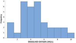
Checkpoint 8.1.3. Describe distribution.

Examine the data from the first year in WaterQuality.txt. Describe the shape, center, and variability of the distribution. In particular, how do the mean and median compare? Do these data appear to be well-modelled by a normal distribution?

🔗

Solution.

The distribution of dissolved oxygen is skewed to the right, centered around 5, with most of the observations between 3 and 8 (\(s = 2.39\) mg/l). The mean (4.735) is larger than the median (4.300). The data are not normally distributed.

🔗

Descriptive statistics and histogram for water quality data

🔗

Checkpoint 8.1.4. State hypotheses.

State the null and alternative hypotheses for testing whether the long-run mean dissolved oxygen in this river is less than 5.0 mg/l (indicating too little oxygen in the water, causing problems in the aquatic community structure).

🔗

Define the parameter:

🔗

\(H_0: \)

🔗

\(H_a: \)

🔗

Solution.

Let \(\mu\) represent the long-run mean dissolved oxygen in this river.

🔗

\(H_0: \mu = 5.0\) mg/l

🔗

\(H_a: \mu < 5.0\) mg/l

🔗

Checkpoint 8.1.5. Assess validity of t-test.

Is the one-sample t-test likely to be valid for these data? Explain why or why not.

🔗

Solution.

The sample size is 34 and the data are not severely skewed so perhaps the t procedures for the population mean will be valid (but not a prediction interval).

🔗

Checkpoint 8.1.6. Calculate proportion non-compliant.

An alternative analysis involves recoding the observations as "compliant" and "not compliant." If we say a measurement is non-compliant when the dissolved oxygen is below 5.0 mg/l, how many non-compliant measurements do we have in this data set? What proportion of the sample is below 5.0 mg/l (non-compliant)?

🔗

Hint.

What do you want to do with the observation that is equal to 5.0?

🔗

Solution.

Nineteen of the 34 measurements are less than 5 (56% "non-compliant"). One observation is equal to 5 (need to decide whether you want to count that as compliant or not).

🔗

Checkpoint 8.1.7. Test proportion non-compliant.

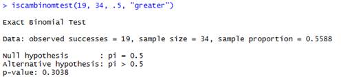
Carry out a test for deciding whether the proportion of measurements that fall below 5.0 mg/l is statistically significantly larger than 0.50 (one-half).

🔗

Solution.

Let \(\pi\) refer to the probability of a non-compliant measurement in this river.

🔗

\(H_0: \pi = 0.50\) vs. \(H_a: \pi > 0.50\text{.}\)

🔗

Assuming independent observations (systematic sample) and a constant probability of success (under the null \(\pi = 0.50\) for this observation period), we can model this with the binomial distribution (\(n = 34\) and \(\pi = 0.50\)).

🔗

\(P(X \geq 19) \approx 0.3038\text{.}\)

🔗

We do not have a small p-value, so we do not have evidence that the probability of non-compliance exceeds 0.50.

🔗

🔗

Checkpoint 8.1.8. Interpret median.

If you decide that more than half of the time the river is non-compliant (that is, more than 50% of measurements are below 5.0 mg/l), what does that imply about the long-run median dissolved oxygen level? Explain.

🔗

Solution.

If more than half of the observations are less than 5.0, this implies that the median is less than 5.0.

🔗

Checkpoint 8.1.9. Compare to t-test.

Identify one advantage to this analysis over the one-sample t-test. Identify one disadvantage of this analysis over the one-sample t-test.

🔗

Advantage:

🔗

Disadvantage:

🔗

Solution.

We do not have to worry about the shape of the sample distribution or the sample size to use the binomial test. However, we only get to talk about whether or not they are non-compliant, not how small the actual observed oxygen levels are.

🔗

Checkpoint 8.1.10. Alternative criterion.

The researchers actually wanted to decide whether the river was non-compliant more than 10% of the time. How would that change your analysis in checkpoint 8.1.7 and would the p-value be larger or smaller?

🔗

Solution.

Now our hypotheses would be \(H_0: \pi = 0.10\) vs. \(H_a: \pi > 0.10\text{.}\) With a sample proportion of 0.5588, our p-value would be much, much smaller in this case.

🔗

Study Conclusions.

Both the mean (not shown) and of the median indicate that dissolved oxygen in this river tended to below the 5.0 mg/l that was cited as the "action level." Although we don’t have statistically significant evidence that the long-run median DO level is below 5.0 mg/l (binomial p-value \(\approx 0.30\)), the researchers actually wanted to engage in remedial action if the river is found to be in non-compliance significantly more than 10% of the time. The exact binomial probability of observing 19 or more non-compliant values from a process with a 0.10 chance of non-compliance is \(4.16 \times 10^{-11}\text{,}\) leaving "little doubt that the 10% non-compliant criterion was exceeded at the monitoring site during 2000."

🔗

Discussion: Sign Test.

When we use 0.50 as the hypothesized probability of success and we count how many of our quantitative observations exceed some pre-specified level, this is called the sign test and corresponds to a test of whether the population median equals that pre-specified level. The sign test can be advantageous over the t-test if the technical conditions for the t-test are not met (e.g., skewness in sample, not a large sample size). However, although this procedure focuses on how often you are above or below that level, it does not provide information about how far above or below as a confidence interval for the mean could.

🔗

Subsection 8.1.1 Practice Problem 2.7

Return to Practice Problem 2.2A and the 30seconds.txt data. Carry out a test to determine whether there is convincing evidence that the median student estimate of 30 seconds differs from 30. (State your hypothesis, statistic and/or standardized statistic, and p-value.)

🔗

Checkpoint 8.1.11.

Carry out the sign test for the 30 seconds data.

🔗

You have attempted of activities on this page.

🔗

Prev Top Next