Problem Solving with Algorithms and Data Structures using C++: The PreTeXt Interactive Edition

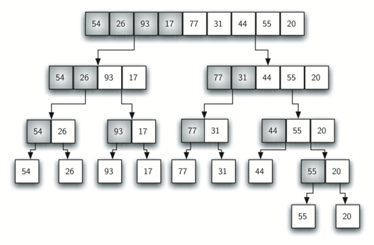
We now turn our attention to using a divide and conquer strategy as a way to improve the performance of sorting algorithms. The first algorithm we will study is the merge sort. Merge sort is a recursive algorithm that continually splits a vector in half. If the vector is empty or has one item, it is sorted by definition (the base case). If the vector has more than one item, we split the vector and recursively invoke a merge sort on both halves. Once the two halves are sorted, the fundamental operation, called a merge, is performed. Merging is the process of taking two smaller sorted vectors and combining them together into a single, sorted, new vector. 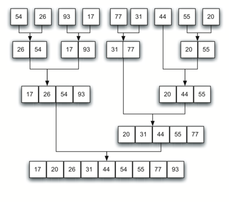Figure 7.7.1 shows our familiar example vector as it is being split by mergeSort. Figure 7.7.2 shows the simple vectors, now sorted, as they are merged back together.

The mergeSort function shown in Task 7.7.1.a begins by asking the base case question. If the length of the vector is less than or equal to one, then we already have a sorted vector and no more processing is necessary. If, on the other hand, the length is greater than one, then we utilize the vector intializer using .begin to extract the left and right halves. This is similar to using the Python slice operation to extract the left and right halves. It is important to note that the vector may not have an even number of items. That does not matter, as the lengths will differ by at most one.

Once the mergeSort function is invoked on the left half and the right half (lines 8–9), it is assumed they are sorted. The rest of the function (lines 11–31) is responsible for merging the two smaller sorted vectors into a larger sorted vector. Notice that the merge operation places the items back into the original vector (avector) one at a time by repeatedly taking the smallest item from the sorted vectors.

The mergeSort function has been augmented with a print statement (line 2) to show the contents of the vector being sorted at the start of each invocation. There is also a print statement (line 32) to show the merging process. The transcript shows the result of executing the function on our example vector. Note that the vector with 44, 55, and 20 will not divide evenly. The first split gives [44] and the second gives [55,20]. It is easy to see how the splitting process eventually yields a vector that can be immediately merged with other sorted vectors.

The visualization in Figure 7.7.3 allows you to step through the algorithm. Red bars represent the element being looked at and blue represents the last element to look at during a pass.

The video in Figure 7.7.4 highlights the individual components of the algorithm itself. The arrows on the bottom indicate the left, middle, and right portions that the algorithm is currently examining. Left and right components are indicated by the color brown, while the middle is indicated by orange. Look for the “divide-and-conquer” aspect of the algorithm here.

In order to analyze the mergeSort function, we need to consider the two distinct processes that make up its implementation. First, the vector is split into halves. We already computed (in a binary search) that we can divide a vector in half \(\log n\) times where n is the length of the vector. The second process is the merge. Each item in the vector will eventually be processed and placed on the sorted vector. So the merge operation which results in a vector of size n requires n operations. The result of this analysis is that \(\log n\) splits, each of which costs \(n\) for a total of \(n\log n\) operations. A merge sort is an \(O(n\log n)\) algorithm.

Recall that the slicing operator is \(O(k)\) where k is the size of the slice. In order to guarantee that mergeSort will be \(O(n\log n)\) we will need to remove the slice operator. Again, this is possible if we simply pass the starting and ending indices along with the vector when we make the recursive call. We leave this as an exercise.

It is important to notice that the mergeSort function requires extra space to hold the two halves as they are extracted with the slicing operations. This additional space can be a critical factor if the vector is large and can make this sort problematic when working on large data sets. In the case with using lists in python, the space complexity is \(O(\log n)\text{.}\)