ads Graphs of Relations on a Set

Section 6.2 Graphs of Relations on a Set

In this section we introduce directed graphs as a way to visualize relations on a set.

Subsection 6.2.1 Digraphs

Let

A = {0, 1, 2, 3},

and let

r = {(0, 0), (0, 3), (1, 2), (2, 1), (3, 2), (2, 0)}

🔗

In representing this relation as a graph, elements of

A

are called the vertices of the graph. They are typically represented by labeled points or small circles. We connect vertex

a

to vertex

b

with an arrow, called an edge, going from vertex

a

to vertex

b

if and only if

a r b .

This type of graph of a relation

r

is called a directed graph or digraph. Figure 6.2.1 is a digraph for

r .

Notice that since 0 is related to itself, we draw a “self-loop” at 0.

described in detail following the image — 🔗
Figure 6.2.1. Digraph of a relation

🔗

The actual location of the vertices in a digraph is immaterial. The actual location of vertices we choose is called an embedding of a graph. The main idea is to place the vertices in such a way that the graph is easy to read. After drawing a rough-draft graph of a relation, we may decide to relocate the vertices so that the final result will be neater. Figure 6.2.1 could also be presented as in Figure 6.2.2.

Digraph of the relation r, alternate embedding — 🔗
Figure 6.2.2. Alternate embedding of the previous directed graph

🔗

A vertex of a graph is also called a node, point, or a junction. An edge of a graph is also referred to as an arc, a line, or a branch. Do not be concerned if two graphs of a given relation look different as long as the connections between vertices are the same in the two graphs.

Example 6.2.3. Another directed graph.

Consider the relation

s

whose digraph is Figure 6.2.4. What information does this give us? The graph tells us that

s

is a relation on

A = {1, 2, 3}

and that

s = {(1, 2), (2, 1), (1, 3), (3, 1), (2, 3), (3, 3)} .

🔗

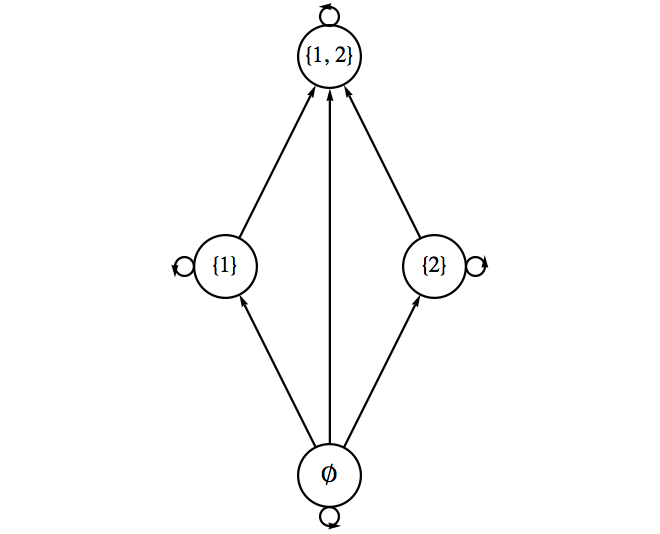
We will be building on the next example in the following section.

Example 6.2.5. Ordering subsets of a two element universe.

Let

B = {1, 2},

and let

A = P (B) = {\emptyset, {1}, {2}, {1, 2}} .

Then

\subseteq

is a relation on

A

whose digraph is Figure 6.2.6.

We will see in the next section that since

\subseteq

has certain structural properties that describe “partial orderings.” We will be able to draw a much simpler type graph than this one, but for now the graph above serves our purposes.

🔗

Exercises 6.2.2 Exercises

🔗

1.

🔗

Let

A = {1, 2, 3, 4},

and let

r

be the relation

\leq

A .

Draw a digraph for

r .

Answer.

🔗

2.

🔗

Let

B = {1, 2, 3, 4, 6, 8, 12, 24},

and let

s

be the relation “divides” on

B .

Draw a digraph for

s .

🔗

3.

🔗

Let

A = {1, 2, 3, 4, 5} .

Define

t

A

a t b

if and only if

b - a

is even. Draw a digraph for

t .

Answer.

See Figure 6.2.8

Figure 6.2.8. Digraph of the relation $t$

🔗

4.

🔗

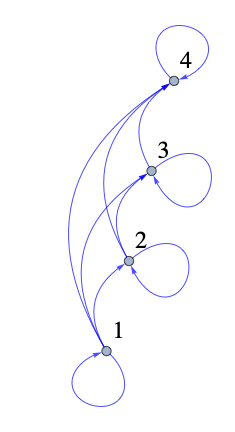
Let

A

be the set of strings of 0’s and 1’s of length 2 or less. This includes the empty string,

λ,

which is the only string of length zero.

Define the relation of $d$ on $A$ by $x d y$ if $x$ is contained within $y .$ For example, $1 d 01 .$ Draw a digraph for this relation.
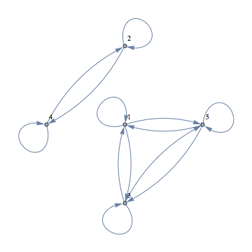
Do the same for the relation $p$ defined by $x p y$ if $x$ is a prefix of $y .$ For example, $1 p 10,$ but $1 p 01$ is false.

🔗

5.

🔗

Recall the relation in Exercise 5 of Section 6.1,

ρ

defined on the power set,

P (S),

of a set

S .

The definition was

(A, B) \in ρ

iff

A \cap B = \emptyset .

Draw the digraph for

ρ

where

S = {a, b} .

🔗

6.

🔗

Let

C = {1, 2, 3, 4, 6, 12},

the divisors of 12, and define

t

C

a t b

if and only if

a

and

b

share a common divisor greater than 1. Draw a digraph for

t .

You have attempted 1 of 1 activities on this page.

Prev Top Next