AC Improper Integrals

Section 6.5 Improper Integrals

Motivating Questions

What are improper integrals and why are they important?
What does it mean to say that an improper integral converges or diverges?
What are some typical improper integrals that we can classify as convergent or divergent?

Another important application of the definite integral measures the likelihood of certain events. For instance, consider a company that manufactures incandescent light bulbs. Based on a large volume of test results, they have determined that the fraction of light bulbs that fail between times

t = a

and

t = b

of use (where

t

is measured in months) is given by

🔗

\int_{a}^{b} 0.3 e^{- 0.3 t} d t .

🔗

For example, the fraction of light bulbs that fail during their third month of use is given by

🔗

\begin{aligned} \int_{2}^{3} 0.3 e^{- 0.3 t} d t & = - e^{- 0.3 t} |_{2}^{3} \\ = - e^{- 0.9} + e^{- 0.6} \\ \approx 0.1422 . \end{aligned}

🔗

Thus about 14.22% of all lightbulbs fail between

t = 2

and

t = 3 .

Clearly we could adjust the limits of integration to measure the fraction of light bulbs that fail during any time period of interest.

🔗

Preview Activity 6.5.1.

A company with a large customer base has a call center that receives thousands of calls a day. After studying the data that represents how long callers wait for assistance, they find that the function

p (t) = 0.25 e^{- 0.25 t}

models the time customers wait in the following way: the fraction of customers who wait between

t = a

and

t = b

minutes is given by

🔗

\int_{a}^{b} p (t) d t .

Use this information to answer the following questions.

🔗

(a) The fraction of callers who wait between 5 and 10 minutes is .

🔗

(b) The fraction of callers who wait between 10 and 20 minutes is .

🔗

(i) What is the fraction of callers who wait between 0 and 5 minutes?

🔗

Answer:

🔗

(ii) What is the fraction of callers who wait between 0 and 10 minutes?

🔗

Answer:

🔗

(iii) Between 0 and 15 minutes?

🔗

Answer:

🔗

(iv) Between 0 and 20?

🔗

Answer:

🔗

(d) Let

F (b)

represent the fraction of callers who wait between

0

and

b

minutes. Find a formula for

F (b)

that involves a definite integral.

🔗

F (b) = \int_{c}^{d} f (t) d t

🔗

where

c =

d =

, and

f (t) =

🔗

Now evaluate that integral using the First FTC to find a formula for

F (b)

that does not involve a definite integral (but will involve

b

🔗

F (b) =

🔗

(e) Calculate

lim_{b \to \infty} F (b) =

🔗

Why does that answer make sense?

🔗

Because one customer is helped at a time.
Because no one waits more than an hour.
Because every customer waits between 0 and infinity minutes.
none of the above

🔗

Subsection 6.5.1 Improper Integrals Involving Unbounded Intervals

In view of the above examples, we see that we may want to integrate over an interval whose upper limit grows without bound. For example, to find the fraction of light bulbs that fail eventually, we wish to find

🔗

lim_{b \to \infty} \int_{0}^{b} 0.3 e^{- 0.3 t} d t,

for which we will also use the notation

🔗

\begin{matrix} (6.5.1) & \int_{0}^{\infty} 0.3 e^{- 0.3 t} d t . \end{matrix}

🔗

Such an integral can be interpreted as the area of an unbounded region, as pictured at right in Figure 6.5.1.

🔗

Figure 6.5.1. At left, the area bounded by $p (t) = 0.3 e^{- 0.3 t}$ on the finite interval $[0, b];$ at right, the result of letting $b \to \infty .$ By “ $\dots$ ” in the righthand figure, we mean that the region extends to the right without bound.
🔗

We call an integral for which the interval of integration is unbounded improper. For instance, the integrals

🔗

\int_{1}^{\infty} \frac{1}{x^{2}} d x, \int_{- \infty}^{0} \frac{1}{1 + x^{2}} d x, and \int_{- \infty}^{\infty} e^{- x^{2}} d x

are all improper because they have limits of integration that involve

\infty .

To evaluate an improper integral we replace it with a limit of proper integrals. That is,

🔗

\int_{0}^{\infty} f (x) d x = lim_{b \to \infty} \int_{0}^{b} f (x) d x .

🔗

We first attempt to evaluate

\int_{0}^{b} f (x) d x

using the First FTC, and then evaluate the limit. Is it even possible for the area of an unbounded region to be finite? The following activity explores this issue and others in more detail.

🔗

Activity 6.5.2.

In this activity we explore the improper integrals

\int_{1}^{\infty} \frac{1}{x} d x

and

\int_{1}^{\infty} \frac{1}{x^{3 / 2}} d x .

🔗

First we investigate $\int_{1}^{\infty} \frac{1}{x} d x .$
1. Use the First FTC to determine the exact values of $\int_{1}^{10} \frac{1}{x} d x,$ $\int_{1}^{1000} \frac{1}{x} d x,$ and $\int_{1}^{100000} \frac{1}{x} d x .$ Then, use your computational device to compute a decimal approximation of each result.
2. Use the First FTC to evaluate the definite integral $\int_{1}^{b} \frac{1}{x} d x$ (which results in an expression that depends on $b$ ).
3. Now, use your work from (ii.) to evaluate the limit given by
  
  $lim_{b \to \infty} \int_{1}^{b} \frac{1}{x} d x .$
Next, we investigate $\int_{1}^{\infty} \frac{1}{x^{3 / 2}} d x .$
1. Use the First FTC to determine the exact values of $\int_{1}^{10} \frac{1}{x^{3 / 2}} d x,$ $\int_{1}^{1000} \frac{1}{x^{3 / 2}} d x,$ and $\int_{1}^{100000} \frac{1}{x^{3 / 2}} d x .$ Then, use your calculator to compute a decimal approximation of each result.
2. Use the First FTC to evaluate the definite integral $\int_{1}^{b} \frac{1}{x^{3 / 2}} d x$ (which results in an expression that depends on $b$ ).
3. Now, use your work from (ii.) to evaluate the limit given by
  
  $lim_{b \to \infty} \int_{1}^{b} \frac{1}{x^{3 / 2}} d x .$
Plot the functions $y = \frac{1}{x}$ and $y = \frac{1}{x^{3 / 2}}$ on the same coordinate axes for the values $x = 0 \dots 10 .$ How would you compare their behavior as $x$ increases without bound? What is similar? What is different?
How would you characterize the value of $\int_{1}^{\infty} \frac{1}{x} d x ?$ of $\int_{1}^{\infty} \frac{1}{x^{3 / 2}} d x ?$ What does this tell us about the respective areas bounded by these two curves for $x \geq 1 ?$

🔗

Subsection 6.5.2 Convergence and Divergence

Activity 6.5.2 suggests that

lim_{b \to \infty} \int_{1}^{b} f (x) d x

is either finite or infinite (or it doesn’t exist). With these possibilities in mind, we introduce the following terminology.

🔗

f (x)

is nonnegative for

x \geq a,

then we say that the improper integral

\int_{a}^{\infty} f (x) d x

converges provided that

🔗

lim_{b \to \infty} \int_{a}^{b} f (x) d x

exists and is finite. Otherwise, we say that

\int_{a}^{\infty} f (x) d x

diverges.

🔗

We will restrict our interest to improper integrals for which the integrand is nonnegative. Also, we require that

lim_{x \to \infty} f (x) = 0,

for if

f

does not approach

0

x \to \infty,

then it is impossible for

\int_{a}^{\infty} f (x) d x

to converge.

🔗

Activity 6.5.3.

Determine whether each of the following improper integrals converges or diverges. For each integral that converges, find its exact value.

🔗

$\int_{1}^{\infty} \frac{1}{x^{2}} d x$
$\int_{0}^{\infty} e^{- x / 4} d x$
$\int_{2}^{\infty} \frac{9}{(x + 5)^{2 / 3}} d x$
$\int_{4}^{\infty} \frac{3}{(x + 2)^{5 / 4}} d x$
$\int_{0}^{\infty} x e^{- x / 4} d x$
$\int_{1}^{\infty} \frac{1}{x^{p}} d x,$ where $p$ is a positive real number

🔗

Subsection 6.5.3 Improper Integrals Involving Unbounded Integrands

An integral is also called improper if the integrand is unbounded on the interval of integration. For example, consider

🔗

\int_{0}^{1} \frac{1}{\sqrt{x}} d x .

Because

f (x) = \frac{1}{\sqrt{x}}

has a vertical asymptote at

x = 0,

f

is not continuous on

[0, 1],

and the integral represents the area of the unbounded region shown at right in Figure 6.5.2.

🔗

Figure 6.5.2. At left, the area bounded by $f (x) = \frac{1}{\sqrt{x}}$ on the finite interval $[a, 1];$ at right, the result of letting $a \to 0^{+},$ where we see that the shaded region will extend vertically without bound.
🔗

We address the problem of the integrand being unbounded by replacing the improper integral with a limit of proper integrals. For example, to evaluate

\int_{0}^{1} \frac{1}{\sqrt{x}} d x,

we replace

0

with

a

and let

a

approach 0 from the right. Thus,

🔗

\int_{0}^{1} \frac{1}{\sqrt{x}} d x = lim_{a \to 0^{+}} \int_{a}^{1} \frac{1}{\sqrt{x}} d x .

We evaluate the proper integral

\int_{a}^{1} \frac{1}{\sqrt{x}} d x,

and then take the limit. We will say that the improper integral converges if this limit exists, and diverges otherwise. In this example, we observe that

🔗

\begin{aligned} \int_{0}^{1} \frac{1}{\sqrt{x}} d x & = lim_{a \to 0^{+}} \int_{a}^{1} \frac{1}{\sqrt{x}} d x \\ = lim_{a \to 0^{+}} {2 \sqrt{x} |}_{a}^{1} \\ = lim_{a \to 0^{+}} 2 \sqrt{1} - 2 \sqrt{a} \\ = 2, \end{aligned}

so the improper integral

\int_{0}^{1} \frac{1}{\sqrt{x}} d x

converges (to the value 2).

🔗

We have to be particularly careful with unbounded integrands, for they may arise in ways that may not initially be obvious. Consider, for instance, the integral

🔗

\int_{1}^{3} \frac{1}{(x - 2)^{2}} d x .

🔗

At first glance we might think that we can simply apply the Fundamental Theorem of Calculus by antidifferentiating

\frac{1}{(x - 2)^{2}}

to get

- \frac{1}{x - 2}

and then evaluating from

1

3 .

Were we to do so, we would be erroneously applying the FTC because

f (x) = \frac{1}{(x - 2)^{2}}

fails to be continuous throughout the interval, as seen in Figure 6.5.3.

🔗

Figure 6.5.3. The function $f (x) = \frac{1}{(x - 2)^{2}}$ on an interval including $x = 2 .$
🔗

Such an incorrect application of the FTC leads to an impossible result (

- 2

), which would itself suggest that something we did must be wrong. Instead, we must address the vertical asymptote at

x = 2

by writing

🔗

\int_{1}^{3} \frac{1}{(x - 2)^{2}} d x = lim_{a \to 2^{-}} \int_{1}^{a} \frac{1}{(x - 2)^{2}} d x + lim_{b \to 2^{+}} \int_{b}^{3} \frac{1}{(x - 2)^{2}} d x .

We then evaluate two separate limits of proper integrals. For instance, doing so for the integral with

a

approaching

2

from the left, we find

🔗

\begin{aligned} \int_{1}^{2} \frac{1}{(x - 2)^{2}} d x & = lim_{a \to 2^{-}} \int_{1}^{a} \frac{1}{(x - 2)^{2}} d x \\ = lim_{a \to 2^{-}} - \frac{1}{(x - 2)} |_{1}^{a} \\ = lim_{a \to 2^{-}} - \frac{1}{(a - 2)} + \frac{1}{1 - 2} \\ = \infty, \end{aligned}

since

\frac{1}{a - 2} \to - \infty

a

approaches 2 from the left. Thus, the improper integral

\int_{1}^{2} \frac{1}{(x - 2)^{2}} d x

diverges; similar work shows that

\int_{2}^{3} \frac{1}{(x - 2)^{2}} d x

also diverges. From either of these two results, we can conclude that that the original integral,

\int_{1}^{3} \frac{1}{(x - 2)^{2}} d x

diverges, too.

🔗

Activity 6.5.4.

For each of the following definite integrals, decide whether the integral is improper or not. If the integral is proper, evaluate it using the First FTC. If the integral is improper, determine whether or not the integral converges or diverges; if the integral converges, find its exact value.

🔗

$\int_{0}^{1} \frac{1}{x^{1 / 3}} d x$
$\int_{0}^{2} e^{- x} d x$
$\int_{1}^{4} \frac{1}{\sqrt{4 - x}} d x$
$\int_{- 2}^{2} \frac{1}{x^{2}} d x$
$\int_{0}^{π / 2} \tan (x) d x$
$\int_{0}^{1} \frac{1}{\sqrt{1 - x^{2}}} d x$

🔗

Subsection 6.5.4 Summary

An integral $\int_{a}^{b} f (x) d x$ can be improper if at least one of $a$ or $b$ is $\pm \infty,$ making the interval unbounded, or if $f$ has a vertical asymptote at $x = c$ for some value of $c$ that satisfies $a \leq c \leq b .$ One reason that improper integrals are important is that certain probabilities can be represented by integrals that involve infinite limits.
When we encounter an improper integral, we work to understand it by replacing the improper integral with a limit of proper integrals. For instance, we write

$\int_{a}^{\infty} f (x) d x = lim_{b \to \infty} \int_{a}^{b} f (x) d x,$

and then work to determine whether the limit exists and is finite. For any improper integral, if the resulting limit of proper integrals exists and is finite, we say the improper integral converges. Otherwise, the improper integral diverges.
An important class of improper integrals is given by

$\int_{1}^{\infty} \frac{1}{x^{p}} d x$

where $p$ is a positive real number. We can show that this improper integral converges whenever $p > 1,$ and diverges whenever $0 < p \leq 1 .$ A related class of improper integrals is $\int_{0}^{1} \frac{1}{x^{p}} d x,$ which converges for $0 < p < 1,$ and diverges for $p \geq 1 .$

🔗

Exercises 6.5.5 Exercises

1.

Calculate the integral below, if it converges. If it does not converge, enter diverges for your answer.

🔗

\int_{2}^{\infty} 4 x e^{- x^{2}} d x =

🔗

2.

Calculate the integral, if it converges. If it diverges, enter diverges for your answer.

🔗

\int_{- \infty}^{- 1} \frac{e^{5 x}}{1 + e^{5 x}} d x =

🔗

3.

Calculate the integral, if it converges. If it diverges, enter diverges for your answer.

🔗

\int_{- 1}^{1} \frac{1}{v} d v =

🔗

4.

Find the area under the curve

y = \frac{1}{\cos^{2} (t)}

between

t = 0

and

t = π / 2 .

Enter diverges if the area is not bounded.

🔗

area =

🔗

5.

Find what value of

c

does

🔗

\int_{4}^{\infty} \frac{c}{x^{3}} d x = 1 ?

🔗

Answer:

🔗

6.

Compute the value of the following improper integral. If it is divergent, type "Diverges" or "D".

🔗

\int_{0}^{2} \frac{d x}{x^{2} - 5 x + 4}

Answer:

🔗

7.

Suppose that a company expects its annual profits

t

years from now to be

f (t)

dollars and that interest is considered to be compounded continuously at an annual rate

r .

Then the present value of all future profits can be shown to be

🔗

F P = \int_{0}^{\infty} e^{- r t} f (t) d t

Find

F P

r = 0.08

and

f (t) = 100, 000 + 1000 t .

🔗

The present value is dollars.

🔗

8.

Radioactive substances decay exponentially: The mass at time

t

m (t) = m (0) e^{k t},

where

m (0)

is the initial mass and

k

is a negative constant. The mean life M of an atom in the substance is

🔗

M = - k \int_{0}^{\infty} t e^{k t} d t .

For the radioactive carbon isotope,

^{14}

C, used in radiocarbon dating, the value of

k

is -0.000121. Find the mean life of a

^{14}

C atom.

🔗

Make sure that your answer is correct to two decimal places.

🔗

M =

🔗

9.

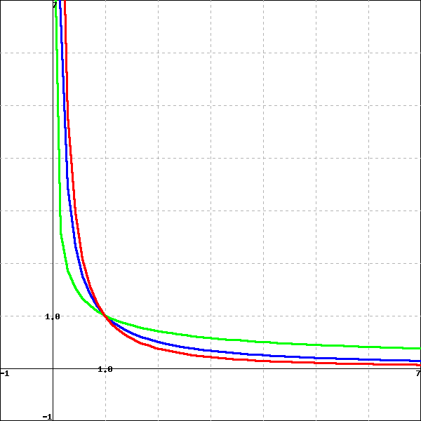
Given the function

f (x) = \frac{1}{x^{1 / 2}}

(in blue), consider the functions

g

(in green) and

h

(in red) graphed below which are continuous on

(0, \infty) .

Assuming the graphs continues in the same way as

x

goes to infinity, answer the following questions.

🔗

choose one
Converge
Diverge
Not sufficient information

1. Does the improper integral

\int_{1}^{\infty} f (x) d x

converge, diverge, or not sufficient information?

🔗

choose one
Converge
Diverge
Not sufficient information

2. Does the improper integral

\int_{1}^{\infty} g (x) d x

converge, diverge, or not sufficient information?

🔗

choose one
Converge
Diverge
Not sufficient information

3. Does the improper integral

\int_{1}^{\infty} h (x) d x

converge, diverge, or not sufficient information?

🔗

Note: You can click on the graph to enlarge the image.

🔗

Note: You only have two attempts at this problem.

🔗

10.

In electromagnetic theory, the magnetic potential

u

at a point on the axis of a circular coil is given by

🔗

u = A r \int_{a}^{\infty} \frac{d x}{(r^{2} + x^{2})^{(3 / 2)}}

where

A, r, a

are constants. Compute

🔗

u

= .

🔗

11.

Determine, with justification, whether each of the following improper integrals converges or diverges.

🔗

$\int_{e}^{\infty} \frac{\ln (x)}{x} d x$
$\int_{e}^{\infty} \frac{1}{x \ln (x)} d x$
$\int_{e}^{\infty} \frac{1}{x (\ln (x))^{2}} d x$
$\int_{e}^{\infty} \frac{1}{x (\ln (x))^{p}} d x,$ where $p$ is a positive real number
$\int_{0}^{1} \frac{\ln (x)}{x} d x$
$\int_{0}^{1} \ln (x) d x$

🔗

12.

Sometimes we may encounter an improper integral for which we cannot easily evaluate the limit of the corresponding proper integrals. For instance, consider

\int_{1}^{\infty} \frac{1}{1 + x^{3}} d x .

While it is hard (or perhaps impossible) to find an antiderivative for

\frac{1}{1 + x^{3}},

we can still determine whether or not the improper integral converges or diverges by comparison to a simpler one. Observe that for all

x > 0,

1 + x^{3} > x^{3},

and therefore

🔗

\frac{1}{1 + x^{3}} < \frac{1}{x^{3}} .

🔗

It therefore follows that

🔗

\int_{1}^{b} \frac{1}{1 + x^{3}} d x < \int_{1}^{b} \frac{1}{x^{3}} d x

for every

b > 1 .

If we let

b \to \infty

so as to consider the two improper integrals

\int_{1}^{\infty} \frac{1}{1 + x^{3}} d x

and

\int_{1}^{\infty} \frac{1}{x^{3}} d x,

we know that the larger of the two improper integrals converges. And thus, since the smaller one lies below a convergent integral, it follows that the smaller one must converge, too. In particular,

\int_{1}^{\infty} \frac{1}{1 + x^{3}} d x

must converge, even though we never explicitly evaluated the corresponding limit of proper integrals. We use this idea and similar ones in the exercises that follow.

🔗

Explain why $x^{2} + x + 1 > x^{2}$ for all $x \geq 1,$ and hence show that $\int_{1}^{\infty} \frac{1}{x^{2} + x + 1} d x$ converges by comparison to $\int_{1}^{\infty} \frac{1}{x^{2}} d x .$
Observe that for each $x > 1,$ $\ln (x) < x .$ Explain why

$\int_{2}^{b} \frac{1}{x} d x < \int_{2}^{b} \frac{1}{\ln (x)} d x$

for each $b > 2 .$ Why must it be true that $\int_{2}^{\infty} \frac{1}{\ln (x)} d x$ diverges?
Explain why $\sqrt{\frac{x^{4} + 1}{x^{4}}} > 1$ for all $x > 1 .$ Then, determine whether or not the improper integral

$\int_{1}^{\infty} \frac{1}{x} \cdot \sqrt{\frac{x^{4} + 1}{x^{4}}} d x$

converges or diverges.

🔗

You have attempted of activities on this page.

🔗

Prev Top Next