How is the instantaneous rate of change of a function at a particular point defined? How is the instantaneous rate of change linked to average rate of change?
The instantaneous rate of change of a function is an idea that sits at the foundation of calculus. It is a generalization of the notion of instantaneous velocity and measures how fast a particular function is changing at a given input. If the original function represents the position of a moving object, this instantaneous rate of change is precisely the instantaneous velocity of the object. In other contexts, instantaneous rate of change could measure the number of cells added to a bacteria culture per day, the number of additional gallons of gasoline consumed per mile by increasing a car’s velocity one mile per hour, or the number of dollars added to a mortgage payment for each percentage point increase in interest rate. The instantaneous rate of change can also be interpreted geometrically on the function’s graph, and this connection is fundamental to many of the main ideas in calculus.
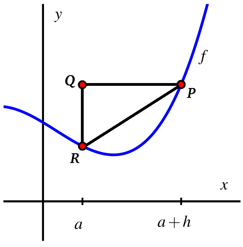
Recall that for a moving object with position function \(s\text{,}\) its average velocity on the time interval \(t = a\) to \(t = a+h\) is given by the quotient
The diagram below shows the graph of a function \(f\) along with points \(P\) and \(R\text{,}\) which lie on the graph. Point \(Q\) is chosen so that \(\triangle PQR\) is a right triangle. (Click on the graph to display a larger version.)
Subsection1.3.2The Derivative of a Function at a Point
Just as we defined instantaneous velocity in terms of average velocity, we now define the instantaneous rate of change of a function at a point in terms of the average rate of change of the function \(f\) over related intervals. This instantaneous rate of change of \(f\) at \(a\) is called “the derivative of \(f\) at \(a\text{,}\)” and is denoted by \(f'(a)\text{.}\)
Let \(f\) be a function and \(x = a\) an input value in the function’s domain. We define the derivative of \(f\) with respect to \(x\) evaluated at \(x = a\), denoted \(f'(a)\text{,}\) by the formula
Aloud, we read the symbol \(f'(a)\) as either “\(f\)-prime at \(a\)” or “the derivative of \(f\) evaluated at \(x = a\text{.}\)” Much of our work in Chapters 1-3 will be devoted to understanding, computing, applying, and interpreting derivatives. For now, we observe the following important things.
The derivative of \(f\) at the value \(x = a\) is defined as the limit of the average rate of change of \(f\) on the interval \([a,a+h]\) as \(h \to 0\text{.}\) This limit may not exist, so not every function has a derivative at every point.
The derivative is a generalization of the instantaneous velocity of a position function: if \(y = s(t)\) is a position function of a moving body, \(s'(a)\) tells us the instantaneous velocity of the body at time \(t=a\text{.}\)
Because the units on \(\frac{f(a+h)-f(a)}{h}\) are “units of \(f(x)\) per unit of \(x\text{,}\)” the derivative has these very same units. For instance, if \(s\) measures position in feet and \(t\) measures time in seconds, the units on \(s'(a)\) are feet per second.
Because the quantity \(\frac{f(a+h)-f(a)}{h}\) represents the slope of the line through \((a,f(a))\) and \((a+h, f(a+h))\text{,}\) when we compute the derivative we are taking the limit of a collection of slopes of lines. Thus, the derivative itself represents the slope of a particularly important line.
When we compute an instantaneous rate of change, we allow the interval \([a,a+h]\) to shrink as \(h \to 0\text{.}\) We can think of one endpoint of the interval as “sliding towards” the other. In particular, provided that \(f\) has a derivative at \((a,f(a))\text{,}\) the point \((a+h,f(a+h))\) will approach \((a,f(a))\) as \(h \to 0\text{.}\) Because the process of taking a limit is a dynamic one, it can be helpful to use computing technology to visualize it. One option is an interactive graphic in which the user is able to control the point that is moving. For a helpful collection of examples, consider the work of David Austin of Grand Valley State University, and this particularly relevant example. For interactives that have been built in Geogebra 1
You can even consider building your own examples; the fantastic program Geogebra is available for free download and is easy to learn and use.
Figure 1.3.4 shows a sequence of figures with several different lines through the points \((a, f(a))\) and \((a+h,f(a+h))\text{,}\) generated by different values of \(h\text{.}\) These lines (shown in the first three figures in magenta), are often called secant lines to the curve \(y = f(x)\text{.}\) A secant line to a curve is simply a line that passes through two points on the curve. For each such line, the slope of the secant line is \(m = \frac{f(a+h) - f(a)}{h}\text{,}\) where the value of \(h\) depends on the location of the point we choose. We can see in the diagram how, as \(h \to 0\text{,}\) the secant lines start to approach a single line that passes through the point \((a,f(a))\text{.}\) If the limit of the slopes of the secant lines exists, we say that the resulting value is the slope of the tangent line to the curve. This tangent line (shown in the right-most figure in green) to the graph of \(y = f(x)\) at the point \((a,f(a))\) has slope \(m = f'(a)\text{.}\)
This figure shows four adjacent graphs of the same function (\(y = f(x) = 0.1 x (x+2) (x-3) + 2\) in the first quadrant) and focuses how we think about identifying the tangent line to graph at \((a,f(a))\text{.}\)
The first image shows the points \((a,f(a))\) and \((a+h,f(a+h))\) where \(h\) is a positive number, as well as the secant line that joins these two points.
The second image again shows the point \((a,f(a))\text{,}\) but now the point \((a+h,f(a+h))\) is adjusted to have \(h\) be about half the size of \(h\) in the first image so that \((a+h,f(a+h))\) is closer on the curve to \((a,f(a))\text{.}\) The secant line that joins \((a,f(a))\) and \((a+h,f(a+h))\) is again shown.
The third image is similar to the first and second. The point\((a,f(a))\) remains fixed, but the point \((a+h,f(a+h))\) is updated again to have \(h\) be about half the size of \(h\) in the second image so that \((a+h,f(a+h))\) is even closer on the curve to \((a,f(a))\text{.}\) Here the points \((a,f(a))\) and \((a+h,f(a+h))\) are very close to one another, andthe secant line that joins them is again shown.
The fourth and final image shows the point \((a,f(a))\) and the tangent line to the curvey \(y = f(x)\) at that point. Up close, the tangent line looks indistinguishable from the curve itself.
If the tangent line at \(x = a\) exists, the graph of \(f\) looks like a straight line when viewed up close at \((a,f(a))\text{.}\) In Figure 1.3.5 we combine the four graphs in Figure 1.3.4 into the single one on the left, and zoom in on the box centered at \((a,f(a))\) on the right. Observe how the tangent line sits relative to the curve \(y = f(x)\) at \((a,f(a))\) and how closely it resembles the curve near \(x = a\text{.}\)
The first image shows the four plots of three secant lines and the tangent line to \(y=f(x)\) on the same graph. There is also a small box centered on the point \((a,f(a))\text{.}\) In this image, especially within the box, the secant lines appear to get closer to the tangent line as \(h\) gets closer to zero.
The second image zooms in on the contents of the box and focuses on the point \((a,f(a))\text{,}\) the tangent line, and the secant line that results from the point \((a+h,f(a+h))\) that is closest to \((a,f(a))\) from the preceding image. The tangent line looks very similar to the curve \(y=f(x)\) (especially near the point \((a,f(a))\)), and the secant line that is shown looks like a just-slightly-tilted version of the tangent line that is not as closely aligned with \(y=f(x)\text{.}\)
Figure1.3.5.A sequence of secant lines approaching the tangent line to \(f\) at \((a,f(a))\text{.}\) At right, we zoom in on the point \((a,f(a))\text{.}\) The slope of the tangent line (in green) to \(f\) at \((a,f(a))\) is given by \(f'(a)\text{.}\)
The instantaneous rate of change of \(f\) with respect to \(x\) at \(x = a\text{,}\)\(f'(a)\text{,}\) also measures the slope of the tangent line to the curve \(y = f(x)\) at \((a,f(a))\text{.}\)
Example1.3.7.Using the limit definition of the derivative.
For the function \(f(x) = x - x^2\text{,}\) use the limit definition of the derivative to compute \(f'(2)\text{.}\) In addition, discuss the meaning of this value and draw a labeled graph that supports your explanation.
Now we use the rule for \(f\text{,}\) and observe that \(f(2) = 2 - 2^2 = -2\) and \(f(2+h) = (2+h) - (2+h)^2\text{.}\) Substituting these values into the limit definition, we have that
Finally, we are able to take the limit as \(h \to 0\text{,}\) and thus conclude that \(f'(2) = -3\text{.}\) We note that \(f'(2)\) is the instantaneous rate of change of \(f\) at the point \((2,-2)\text{.}\) It is also the slope of the tangent line to the graph of \(y = x - x^2\) at the point \((2,-2)\text{.}\)Figure 1.3.8 shows both the function and the line through \((2,-2)\) with slope \(m = f'(2) = -3\text{.}\)
This figure shows a graph of the quadratic function \(y = x - x^2\) along with its tangent line at the point \((2,-2)\text{.}\) The values of \(x\) range horizontally from \(-1\) to \(3\text{;}\) values of \(y\) range vertically from \(-6\) to \(1\text{.}\) The grid boxes are \(1 \times 1\text{.}\)
The graph of \(y = x - x^2\) is a parabola that opens down with vertex at \((\frac12, \frac14)\) and \(x\)-intercepts at \((0,0)\) and \((1,0)\text{.}\) The tangent line passes through \((2,-2)\) on the curve and has slope \(m = -3\text{.}\) Near \(x=2\text{,}\) the curve and the tangent line align perfectly and look indistinguishable.
Compute the average rate of change of \(f\) on the intervals \([1,4]\text{,}\)\([3,7]\text{,}\) and \([5,5+h]\text{;}\) simplify each result as much as possible. What do you notice about these quantities?
Use the limit definition of the derivative to compute the exact instantaneous rate of change of \(f\) with respect to \(x\) at the value \(a = 1\text{.}\) That is, compute \(f'(1)\) using the limit definition. Show your work. Is your result surprising?
A water balloon is tossed vertically in the air from a window. The balloon’s height in feet at time \(t\) in seconds after being launched is given by \(s(t) = -16t^2 + 16t + 32\text{.}\) Use this function to respond to each of the following questions.
A coordinate grid for plotting the function and its tangent line. The values of \(t\) range horizontally from \(-0.5\) to \(2.5\text{;}\) values of \(y\) range vertically from \(-8\) to \(40\text{.}\)
Compute the average rate of change of \(s\) on the time interval \([1,2]\text{.}\) Include units on your answer and write one sentence to explain the meaning of the value you found.
Use the limit definition to compute the instantaneous rate of change of \(s\) with respect to time, \(t\text{,}\) at the instant \(a = 1\text{.}\) Show your work using proper notation, include units on your answer, and write one sentence to explain the meaning of the value you found.
On your graph in (a), sketch two lines: one whose slope represents the average rate of change of \(s\) on \([1,2]\text{,}\) the other whose slope represents the instantaneous rate of change of \(s\) at the instant \(a=1\text{.}\) Label each line clearly.
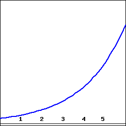
A rapidly growing city in Arizona has its population \(P\) at time \(t\text{,}\) where \(t\) is the number of decades after the year 2010, modeled by the formula \(P(t) = 25000 e^{t/5}\text{.}\) Use this function to respond to the following questions.
A grid an axes for plotting the function \(P(t)\) in the first quadrant. The grid is \(6\) units wide and tall, with no labeled scale, and the coordinate axes lie one unit up from the bottom and one unit in from the left.
Compute the average rate of change of \(P\) between 2030 and 2050. Include units on your answer and write one sentence to explain the meaning (in everyday language) of the value you found.
Use the limit definition to write an expression for the instantaneous rate of change of \(P\) with respect to time, \(t\text{,}\) at the instant \(a = 2\text{.}\) Explain why this limit is difficult to evaluate exactly.
Estimate the limit in (c) for the instantaneous rate of change of \(P\) at the instant \(a = 2\) by using several small \(h\) values. Once you have determined an accurate estimate of \(P'(2)\text{,}\) include units on your answer, and write one sentence (using everyday language) to explain the meaning of the value you found.
On your graph, sketch two lines: one whose slope represents the average rate of change of \(P\) on \([2,4]\text{,}\) the other whose slope represents the instantaneous rate of change of \(P\) at the instant \(a=2\text{.}\)
In a carefully-worded sentence, describe the behavior of \(P'(a)\) as \(a\) increases in value. What does this reflect about the behavior of the given function \(P\text{?}\)
The average rate of change of a function \(f\) on the interval \([a,b]\) is \(AV_{[a,b]} = \frac{f(b)-f(a)}{b-a}\text{.}\) The units on the average rate of change are “units of \(f(x)\) per unit of \(x\)”, and the numerical value of the average rate of change represents the slope of the secant line between the points \((a,f(a))\) and \((b,f(b))\) on the graph of \(y = f(x)\text{.}\) If we view the interval as being \([a,a+h]\) instead of \([a,b]\text{,}\) the meaning is still the same, but the average rate of change is now computed by \(AV_{[a,b]} = \frac{f(a+h)-f(a)}{h}\text{.}\)
The instantaneous rate of change with respect to \(x\) of a function \(f\) at a value \(x = a\) is denoted \(f'(a)\) (read “the derivative of \(f\) evaluated at \(a\)” or “\(f\)-prime at \(a\)”) and is defined by the formula
provided the limit exists. Note particularly that the instantaneous rate of change at \(x = a\) is the limit of the average rate of change on \([a,a+h]\) as \(h \to 0\text{,}\) and that its units are also “units of \(f(x)\) per unit of \(x\)”.
Provided the derivative \(f'(a)\) exists, its value tells us the instantaneous rate of change of \(f\) with respect to \(x\) at \(x = a\text{,}\) which geometrically is the slope of the tangent line to the curve \(y = f(x)\) at the point \((a,f(a))\text{.}\) We even say that \(f'(a)\) is the “slope of the curve” at the point \((a,f(a))\text{.}\)
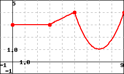
Graph of a piecewise function consisting of a horizontal line on \(0\leq x \leq 3\text{,}\) a nonhorizontal line on \(3\leq x \leq 5\text{,}\) and a parabola on \(5\leq x \leq 9\) with the vertex of the parabola occurring at \(x=7\text{.}\)
E. the derivative of the function is approximately the same as the derivative at \(x = 0.75\) (be sure that you give a point that is distinct from \(x = 0.75\text{!}\)): \(x =\)
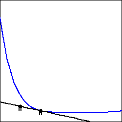
The figure below shows a function \(g(x)\) and its tangent line at the point \(B = (4.8,5.6)\text{.}\) If the point \(A\) on the tangent line is \((4.74,5.64)\text{,}\) fill in the blanks below to complete the statements about the function \(g\) at the point \(B\text{.}\)
Graph of a sharply concave down function with a steep initial slope, bending down as the x-values increase. The point B is on the curve near the initial bend, the tangent line extends through B, and the point A is on the tangent line to the left of B.
What is the approximate value of the average rate of change of \(f\) on \([-3,-1]\text{?}\) On \([0,2]\text{?}\) How are these values related to your work in (a)?
What is the approximate value of the instantaneous rate of change of \(f\) at \(x = -3\text{?}\) At \(x = 0\text{?}\) How are these values related to your work in (a)?
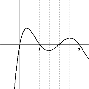
Plot of \(f(x)=0.1 x (x+2) (x-3) + 2\) on the interval \(-5 \lt x \lt 5\text{.}\) The \(y\)-values also are shown on the interval \(-5 \lt y \lt 5\text{.}\)
Two adjacent coordinate axes for plotting the described functions. Each grid has \(x\) ranging horizontally from \(-3.5\) to \(-3.5\text{,}\) and \(y\) ranging vertically from \(-3.5\) to \(-3.5\text{.}\)
Suppose that the population, \(P\text{,}\) of China (in billions) can be approximated by the function \(P(t) = 1.15(1.014)^t\) where \(t\) is the number of years since the start of 1993.
According to the model, what was the total change in the population of China between January 1, 1993 and January 1, 2000? What will be the average rate of change of the population over this time period? Is this average rate of change greater or less than the instantaneous rate of change of the population on January 1, 2000? Explain and justify, being sure to include proper units on all your answers.
Write an expression involving limits that, if evaluated, would give the exact instantaneous rate of change of the population on today’s date. Then estimate the value of this limit (discuss how you chose to do so) and explain the meaning (including units) of the value you have found.
The goal of this problem is to compute the value of the derivative at a point for several different functions, where for each one we do so in three different ways, and then to compare the results to see that each produces the same value.
For each of the following functions, use the limit definition of the derivative to compute the value of \(f'(a)\) using three different approaches: strive to use the algebraic approach first (to compute the limit exactly), then test your result using numerical evidence (with small values of \(h\)), and finally plot the graph of \(y = f(x)\) near \((a,f(a))\) along with the appropriate tangent line to estimate the value of \(f'(a)\) visually. Compare your findings among all three approaches; if you are unable to complete the algebraic approach, still work numerically and graphically.