Section 10.9 Implementing Breadth-First Search
With the graph constructed we can now turn our attention to the algorithm we will use to find the shortest solution to the word ladder problem. The graph algorithm we are going to use is called the breadth-first search (BFS), and it is one of the easiest algorithms for searching a graph. It also serves as a prototype for several other important graph algorithms that we will study later.
Given a starting vertex \(s\) of a graph \(G\text{,}\) a breadth first search proceeds by exploring edges in the graph to find all the vertices in \(G\) for which there is a path from \(s\text{.}\) The remarkable thing about a breadth-first search is that it finds all the vertices that are a distance \(k\) from \(s\) before it finds any vertices that are a distance \(k+1\text{.}\) One good way to visualize what the breadth-first search algorithm does is to imagine that it is building a tree, one level of the tree at a time. A breadth first search adds all children of the starting vertex before it begins to discover any of the grandchildren.
The BFS algorithm creates two new maps.
distance stores how far each vertex is from the starting point. The map previous stores, for each vertex, the previous vertex in the search.
BFS needs to keep track of its progress, in that it needs to know which vertices it has already visited. The map
previous is useful for this. It starts off empty, indicating that no vertices have yet been visited. As we visit vertices, we will add them to the previous map, storing within it which vertex we had previously been visiting.
BFS needs to return both of these maps to the caller. There are multiple approaches for returning multiple values within Kotlin. We use an approach here where we create a new class named
BfsSolver, which stores the maps as instance variables. We then use the init method of the class to call a method that actually runs the algorithm. This approach will have further benefit later on this chapter.
The breadth-first search algorithm shown in Listing 10.9.1 below uses the adjacency list graph representation we developed earlier. In addition it uses a queue, a crucial point as we will see, to decide which vertex to explore next.
class BfsSolver<V>(val graph: GraphADT<V>, val start: V) {
    val previous = mutableMapOf<V, V?>()
    val distance = mutableMapOf<V, Int>()

    init {
        bfs(start)
    }

    private fun bfs(start: V) {
        previous[start] = null
        distance[start] = 0
        val queue = ListQueue<V>()
        queue.enqueue(start)
        while (queue.size() > 0) {
            val current = queue.dequeue()
            val neighbors = graph.getNeighbors(current)!!
            for (neighbor in neighbors) {
                if (neighbor !in previous) {
                    previous[neighbor] = current
                    distance[neighbor] = distance[current]!! + 1
                    queue.enqueue(neighbor)
                }
            }
        }
    }
}
BFS begins by adding the start vertex to the map
previous with a value of null to indicate that no other vertex came before it, and to record that we have visited this vertex. Likewise, we add the starting vertex to the distance map with a value of 0. We create a queue, and then add our starting vertex to that queue. The next step is to begin to systematically explore vertices at the front of the queue. We explore each new node at the front of the queue by iterating over its neighbors. As each neighboring vertex is examined, we check to see if it had previously been visited. If it had not been visited previously, the following things happen:
-
The new unexplored vertex
neighboris added toprevious, with its predecessor set to the current vertexcurrent. -
The distance to
neighborbecomes the distance tocurrentplus one. -
neighboris added to the end of the queue. This schedules this node for further exploration, but not until all the other vertices on the adjacency list ofcurrenthave been explored.
Let’s look at a visual example. When showing BFS visually, colors are commonly used to indicate the state of each vertex. We’ll follow that standard. Each vertex can be white, gray, or black. All the vertices are initialized to white when they are constructed. A white vertex is an undiscovered vertex. When a vertex is initially discovered it is colored gray, and when BFS has completely explored a vertex it is colored black. This means that once a vertex is colored black, it has no white vertices adjacent to it. A gray node, on the other hand, may have some white vertices adjacent to it, indicating that there are still additional vertices to explore.
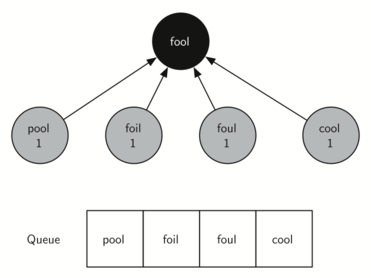
We’ll look in particular at how the
bfs method would construct the breadth-first tree corresponding to the graph in Section 10.8. Starting from FOOL we visit all nodes that are adjacent to FOOL, and add them to the tree. The adjacent nodes include POOL, FOIL, FOUL, and COOL. For each of these nodes, we record their previous vertex (shown via arrows), and their distance (shown as 1). These nodes are then added to the queue of new nodes to explore. Figure 10.9.2 shows the state of the in-progress tree along with the queue after this step. In the figure, the start node is shown as black because we have now discovered all of its neighbors, whereas all of the new nodes are gray because we have not finished exploring each of them.
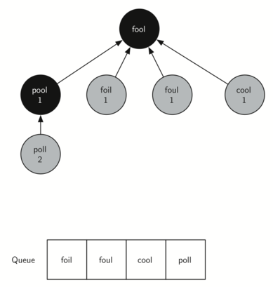
In the next step
bfs removes the next node (POOL) from the front of the queue and repeats the process for all of its adjacent nodes. However, when bfs examines the node COOL, it finds that the color of COOL has already been changed to gray. This indicates that there is a shorter path to COOL and that COOL is already on the queue for further exploration. The only new node added to the queue while examining POOL is POLL. The new state of the tree and queue is shown in Figure 10.9.3.
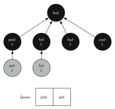
The next vertex on the queue is FOIL. The only new node that FOIL can add to the tree is FAIL. As
bfs continues to process the queue, neither of the next two nodes adds anything new to the queue or the tree. Figure 10.9.4 shows the tree and the queue after expanding all the vertices on the second level of the tree.
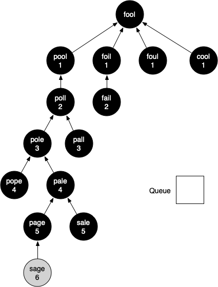
You should continue to work through the algorithm on your own so that you are comfortable with how it works. Figure 10.9.5 shows the final breadth-first search tree after all the vertices in Section 10.8 have been expanded. The amazing thing about the breadth-first search solution is that we have not only solved the FOOL–SAGE problem we started out with, but we have solved many other problems along the way. We can start at any vertex in the breadth-first search tree and follow the predecessor arrows back to the root to find the shortest word ladder from any word back to FOOL.
Listing 10.9.6 shows a
main function for testing the preceding code. After generating a BfsSolver object (which internally calls bfs), the code starts at the end vertex and follows the predecessor links to print out the word ladder, in reverse order.
fun main() {
    val graph = buildGraph("words.txt")

    val startWord = "fool"
    val endWord = "sage"

    val bfsSolution = BfsSolver(graph, startWord)

    // Traverse backwards from end word
    var current: String? = endWord
    while (current != null) {
        println(current)
        current = bfsSolution.previous[current]
    }
}
Here is the output:
sage
sale
pale
pall
poll
pool
fool
You have attempted of activities on this page.
