Section 11.4 Trees Revisited: Quantizing Images
Next to text, digital images are the most common element found on the internet. However, the internet would feel much slower if every advertisement-sized image required 196,560 bytes of memory. Instead, a banner ad image requires only 14,246 bytes, just 7.2% of what it could take. Where do these numbers come from? How is such a phenomenal savings achieved? The answers to these questions are the topic of this section.
Subsection 11.4.1 A Quick Review of Digital Images
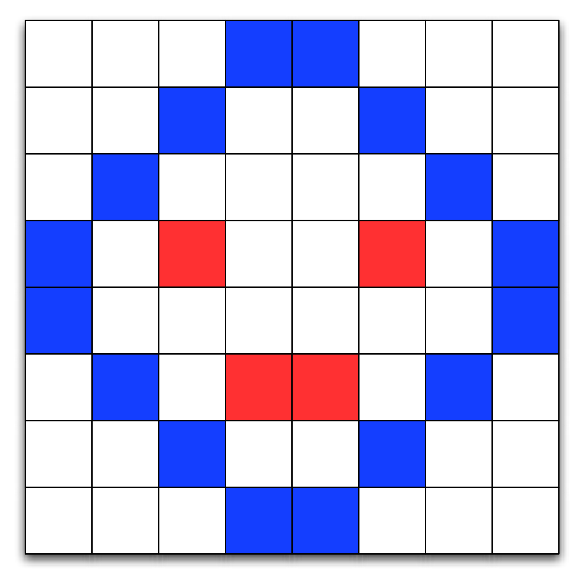
A digital image is composed of thousands of individual components called pixels. The pixels are arranged as a rectangle that forms the image. Each pixel in an image represents a particular color in the image. On a computer, the color of each pixel is determined by a mixture of three primary colors: red, green, and blue. A simple example of how pixels are arranged to form a picture is shown in Figure 11.4.1.
In the physical world colors are not discrete quantities. The colors in our physical world have an infinite amount of variation to them. Just as computers must approximate floating point numbers, they also must approximate the colors in an image. The human eye can distinguish between 200 different levels in each of the three primary colors, or a total of about 8 million individual colors. In practice we use one byte (8 bits) of memory for each color component of a pixel. Eight bits gives us 256 different levels for each of the red, green, and blue components, for a total of 16.7 million different possible colors for each pixel. While the huge number of colors allows artists and graphic designers to create wonderfully detailed images, the downside of all of these color possibilities is that image size grows very rapidly. For example, a single image from a one-megapixel camera would take 3 megabytes of memory.
To represent this image, we might use a list of lists. The list of lists representation of the first two rows of the image in Figure 11.4.1 is shown below:
im = [[(255,255,255),(255,255,255),(255,255,255),(12,28,255),
      (12,28,255),(255,255,255),(255,255,255),(255,255,255),],
      [(255,255,255),(255,255,255),(12,28,255),(255,255,255),
       (255,255,255),(12,28,255),(255,255,255),(255,255,255)],
 ... ]
The color white is represented by \((255, 255, 255)\text{.}\) A bluish color is represented by \((12, 28, 255)\text{.}\)
With this representation for an image in mind, you can imagine that it could be stored in a file by perhaps writing a line for each pixel, and three integers on each line. In practice, many approaches exist, but they are all in general some kind of variaiton on this idea. The key point that is relevant here is that a basic approach for representing the image has to store three numbers for each pixel individually, which can take up a lot of space.
Subsection 11.4.2 Quantizing an Image
There are many ways of reducing the storage requirements for an image. One of the easiest ways is to use fewer colors. Fewer color choices means fewer bits for each red, green, and blue component, which means reduced memory requirements. In fact, one of the most popular image formats used for images on the World Wide Web uses only 256 colors for an image. Using 256 colors reduces the storage requirements from three bytes per pixel to one byte per pixel.
Right now you are probably asking yourself how to take an image that may have as many as 16 million colors and reduce it to just 256? The answer is a process called quantization. To understand the process of quantization, let’s think about colors as a three-dimensional space. Each color can be represented by a point in space where the red component is the x axis, the green component is the y axis, and the blue component is the z axis. We can think of the space of all possible colors as a \(256 \times 256 \times 256\) cube. The colors closest to the vertex at \((0, 0, 0)\) are going to be black and dark color shades. The colors closest to the vertex at \((255, 255, 255)\) are bright and close to white. The colors closest to \((255, 0, 0)\) are red and so forth.
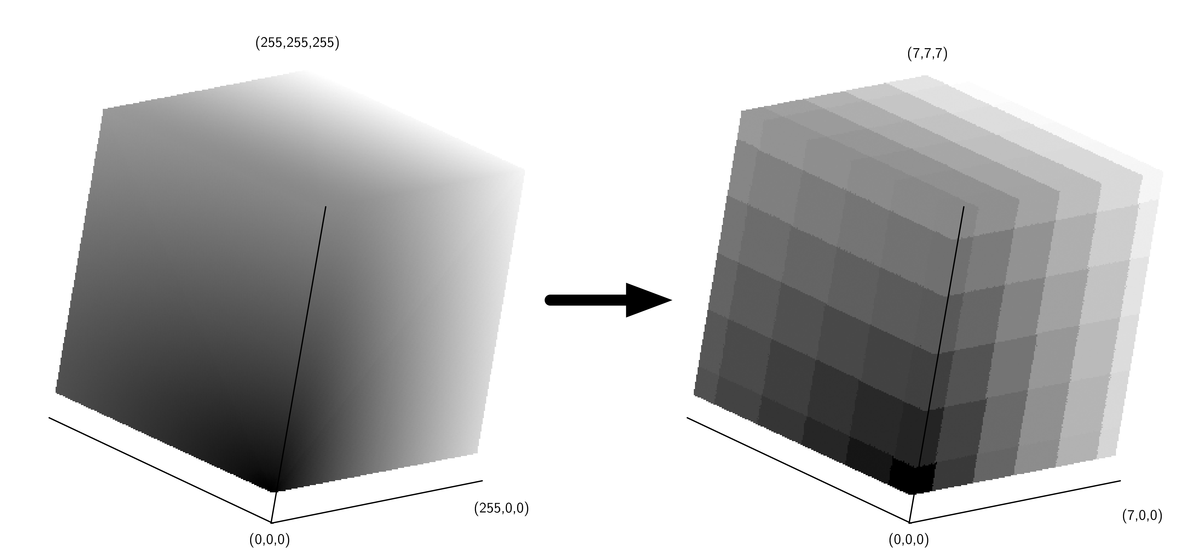
The simplest way to think about quantizing an image is to imagine taking the \(256 \times 256 \times 256\) cube and turning it into an \(8 \times 8 \times 8\) cube. The overall size of the cube stays the same, but now many colors in the old cube are represented by a single color in the new cube. Figure 11.4.2 shows an example of the quantization just described.
We can turn this simple idea of color quantization into the program shown in Listing 11.4.3. The
simpleQuant algorithm works by mapping the color components for each pixel represented by its full 256 bits to the color at the center of the cube in its area. This is easy to do using integer division. In the simpleQuant algorithm there are seven distinct values in the red dimension and six distinct values in the green and blue dimensions.
import java.awt.image.BufferedImage
import javax.swing.JFrame
import javax.swing.WindowConstants

fun simpleQuant(img: BufferedImage) {
    for (row in 0..<img.height) {
        for (col in 0..<img.width) {
            val argb = img.getRGB(col, row)
            var r = (argb shr 16) and 0xff
            var g = (argb shr 8) and 0xff
            var b = argb and 0xff
            r = r / 36 * 36
            g = g / 42 * 42
            b = b / 42 * 42
            img.setRGB(col, row, (r shl 16 or (g shl 8) or b))
        }
    }
}

fun main() {
    print("File name: ")
    val filename = readln()
    val f = JFrame("Simple Quantize")
    f.defaultCloseOperation = WindowConstants.DISPOSE_ON_CLOSE
    val img = ImageComponent(filename)
    simpleQuant(img.image)
    f.add(img)
    f.pack()
    f.isVisible = true
}
Lines 9–11 use bit manipulation to extract the red, green, and blue values. The
shr operator is the right shift operation. and and or are different from && and || in that they are bitwise operators. Bitwise operations work just like the logical operations used in conditionals, except that they work on the individual bits of a number. The shift operation moves the bits \(n\) places to the right, filling in with zeros on the left and dropping the bits as they go off the right.
In line 15,
shl shifts the revised values left. This fills in with zeros on the right an drops bits as they move go off the left. The bitwise or operator puts the new color value back together.
The
main function prompts you for a file name. Line 25 then creates a new ImageComponent, given a file name. This is a class we have also written. It is listed in Listing 11.4.4 for your reference:
ImageComponent Classimport java.awt.Dimension
import java.awt.Graphics
import java.awt.image.BufferedImage
import java.io.File
import javax.imageio.ImageIO
import javax.swing.JComponent
class ImageComponent(filename: String) : JComponent() {
var image: BufferedImage = ImageIO.read(File(filename))
override fun paint(g: Graphics) {
g.drawImage(image, 0, 0, null)
}
override fun getPreferredSize(): Dimension {
return Dimension(
image.getWidth(null),
image.getHeight(null)
)
}
}
This class initializes an instance variable named
image as a BufferedImage object. Lines 11–21 provide methods that the graphics system will call when it needs to display the component and find how large it is.
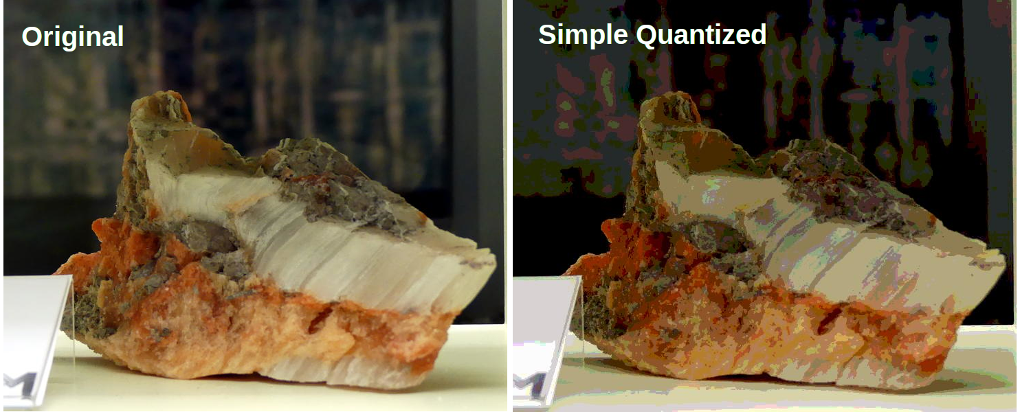
Figure 11.4.5 shows a before and after comparison of original and quantized images of a crystal. You can use any JPEG color image from your collection and run the program to see the differences. Notice how much detail is lost in the quantized picture.
Aside
Subsection 11.4.3 An Improved Quantization Algorithm Using Octrees
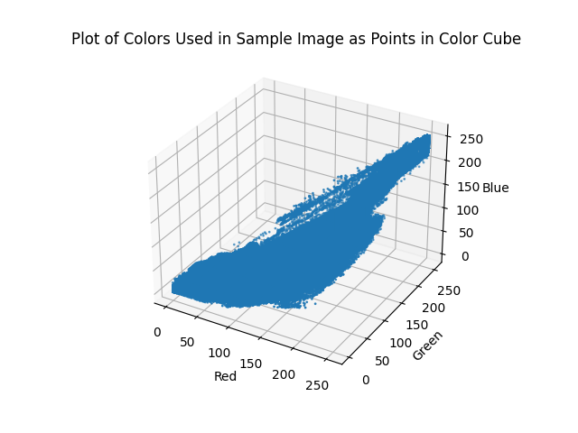
The problem with the simple method of quantization just described is that the colors in most pictures are not evenly distributed throughout the color cube. Many colors may not appear in the image, so parts of the cube may go completely unused. Allocating an unused color to the quantized image is a waste. Figure 11.4.6 shows the distribution of the colors that are used in the example image. Notice how little of the color cube space is actually used.
To make a better quantized image we need to find a way to do a better job of selecting the set of colors we want to use to represent our image. There are several algorithms for dividing the color cube in different ways to allow for the better use of colors. In this section we are going to look at a tree-based solution. The tree solution we will use makes use of an octree. An octree is similar to a binary tree; however, each node in an octree has eight children. Here is the interface we will implement for our octree abstract data type:
-
Octree()creates a new empty octree. -
insert(r, g, b)adds a new node to the octree using the red, green, and blue color values as the key. -
find(r, g, b)finds an existing node, or the closest approximation, using the red, green, and blue color values as the search key. -
reduce(n)reduces the size of the octree so that there are \(n\) or fewer leaf nodes.
Here is how an octree is used to divide the color cube:
-
The root of the octree represents the entire cube.
-
The second level of the octree represents a single slice through each dimension (\(x\text{,}\) \(y\text{,}\) and \(z\)) that evenly divides the cube into eight pieces.
-
The next level of the tree divides each of the eight sub-cubes into eight additional cubes for a total of 64 cubes. Notice that the cube represented by the parent node totally contains all of the sub-cubes represented by the children. As we follow any path down the tree we are staying within the boundary of the parent, but getting progressively more specific about the portion of the cube.
-
The eighth level of the tree represents the full resolution of 16.7 million colors in our color cube.
Now that you know how we can represent the color cube using an octree, you may be thinking that the octree is just another way to divide up the color cube into even parts. You are correct. However, because the octree is hierarchical, we can take advantage of the hierarchy to use larger cubes to represent unused portions of the color cube and smaller cubes to represent the popular colors. Here is an overview of how we will use an octree to do a better job of selecting a subset of the colors in an image:
-
For each pixel in the image:
-
Search for the color of this pixel in the octree. The color will be a leaf node at the eighth level.
-
If the color is not found create a new leaf node at the eighth level (and possibly some internal nodes above the leaf).
-
If the color is already present in the tree increment the counter in the leaf node to keep track of how many pixels are this color.
-
-
Repeat until the number of leaf nodes is less than or equal to the target number of colors.
-
Find the deepest leaf node with the smallest number of uses.
-
Merge the leaf node and all of its siblings together to form a new leaf node.
-
-
The remaining leaf nodes form the color set for this image.
-
To map an original color to its quantized value, search down the tree until you get to a leaf node. Return the color values stored in the leaf.
The ideas outlined above quantize an image are encoded in the Kotlin function
octreeQuant(), shown in Listing 11.4.7.
import java.awt.image.BufferedImage

fun octreeQuant(img: BufferedImage) {
    val w = img.width
    val h = img.height

    val ot: Octree = Octree()
    for (row in 0..<h) {
        for (col in 0..<w) {
            val argb = img.getRGB(col, row)
            val r = (argb shr 16) and 0xff
            val g = (argb shr 8) and 0xff
            val b = argb and 0xff
            ot.insert(r, g, b)
        }
    }

    ot.reduce(256)

    for (row in 0..<h) {
        for (col in 0..<w) {
            val argb = img.getRGB(col, row)
            val r = (argb shr 16) and 0xff
            val g = (argb shr 8) and 0xff
            val b = argb and 0xff

            val newRgb = ot.find(r, g, b)!!

            img.setRGB(
                col, row, (newRgb.red shl 16 or (
                        newRgb.green shl 8) or newRgb.blue)
            )
        }
    }
}
The
octreeQuant function implements the basic process just described. First, the loops in lines 8–16 Listing 11.4.7 read each pixel and add it to the octree. Second, the number of leaf nodes is reduced by the reduce method on line 18. Finally, the image is updated by searching for a color, using find, in the reduced octree on line 27.
Let us now turn our attention to the definition of the
Octree class (Listing 11.4.8), which is where all the magic happens.
Octree Classdata class Pixel(var red: Int, var green: Int, var blue: Int)
class Octree {
var root: OTNode? = null
var numLeaves = 0
var maxLevel = 5
var allLeaves: MutableList<OTNode> = mutableListOf()
fun insert(r: Int, g: Int, b: Int) {
if (this.root == null) {
this.root = OTNode(outer = this)
}
this.root!!.insert(r, g, b, 0, this)
}
fun find(r: Int, g: Int, b: Int): Pixel? {
if (this.root != null) {
return this.root!!.find(r, g, b, 0)
} else {
return null
}
}
fun reduce(maxCubes: Int) {
System.err.printf(
"Reducing %d to %d%n",
this.allLeaves.size, maxCubes
)
while (this.allLeaves.size > maxCubes) {
val smallest = this.findMinCube()
smallest!!.parent!!.merge()
this.allLeaves.add(smallest.parent)
this.numLeaves += 1
}
}
fun findMinCube(): OTNode? {
var minCount = Int.Companion.MAX_VALUE
var maxLevel = 0
var minCube: OTNode? = null
for (node in allLeaves) {
if (node.count <= minCount && node.level >= maxLevel) {
minCube = node
minCount = node.count
maxLevel = node.level
}
}
return minCube
}
}
First notice that the constructor for an
Octree initializes the root node to null. Then it sets up three important attributes that all the nodes of an octree may need to access. Those attributes are maxLevel, numLeaves, and allLeaves. The maxLevel attribute limits the total depth of the tree. Notice that in our implementation we have initialized maxLevel to five. This is a small optimization that allows us to ignore the two least significant bits of color information. It keeps the overall size of the tree much smaller and doesn’t hurt the quality of the final image at all. The numLeaves and allLeaves attributes allow us to keep track of the number of leaf nodes and allow us direct access to the leaves without traversing all the way down the tree. We will see why this is important shortly.
The
insert and find methods behave exactly like their cousins in chapter Chapter 7. They each check to see if a root node exists, and then call the corresponding method in the root node. Notice that insert and find both use the red, green, and blue components ((r, g, b)) to identify a node in the tree.
The
reduce method is defined on line 24 of Listing 11.4.8. This method loops until the number of leaves in the leaf list is less than the total number of colors we want to have in the final image (defined by the parameter maxCubes). reduce makes use of a helper method findMinCube to find the node in the octree with the smallest reference count. Once the node with the smallest reference count is found, that node is merged into a single node with all of its siblings (see line 31 of Listing 11.4.8).
The
findMinCube method is implemented using the allLeaves and a simple find minimum loop pattern. When the number of leaf nodes is large, and it could be as large is 16.7 million, this approach is not very efficient. In one of the exercises you are asked to modify the Octree class and improve the efficiency of findMinCube.
One of the things to mention about the
Octree class is that it uses an instance of the class OTNode which is defined inside the the Octree class. A class that is defined inside another class is called an inner class. We define OTNode inside Octree because each node of an octree needs to have access to some information that is stored in an instance of the Octree class. Another reason for making OTNode an inner class is that there is no reason for any code outside of the Octree class to use it. The way that an octree node is implemented is really a private detail that nobody else needs to know about. This is a good software engineering practice known as information hiding.
Now let’s look at the class definition for the nodes in an octree (Listing 11.4.9). The constructor for the
OTNode class has three parameters: parent, level, and outer. These parameters allow the Octree methods to construct new nodes under a variety of circumstances. As we did with binary search trees, we will keep track of the parent of a node explicitly. The level of the node simply indicates its depth in the tree. The most interesting of these three parameters is the outer parameter, which is a reference to the instance of the octree class that created this node. outer will function like this in that it will allow the instances of OTNode to access attributes of an instance of Octree.
The other attributes that we want to remember about each node in an
octree include the reference count and the red, green, and blue components of the color represented by this tree. As you will note in the insert method, only a leaf node of the tree will have values for red, green, blue, and count. Also note that since each node can have up to eight children we initialize a list of eight references to keep track of them all. Rather than a left and right child as in binary trees, an octree has 0–7 children.
class OTNode(
    val parent: OTNode? = null,
    val level: Int = 0,
    val outer: Octree? = null
) {
    var red = 0
    var green = 0
    var blue = 0
    var count = 0
    val children: MutableList<OTNode?> = MutableList(8) { null }
Now we get into the really interesting parts of the octree implementation. The Java code for inserting a new node into an octree is shown in Listing 11.4.10. The first problem we need to solve is how to figure out where to place a new node in the tree. In a binary search tree we used the rule that a new node with a key less than its parent went in the left subtree, and a new node with a key greater than its parent went in the right subtree. But with eight possible children for each node it is not that simple. In addition, when indexing colors it is not obvious what the key for each node should be. In an
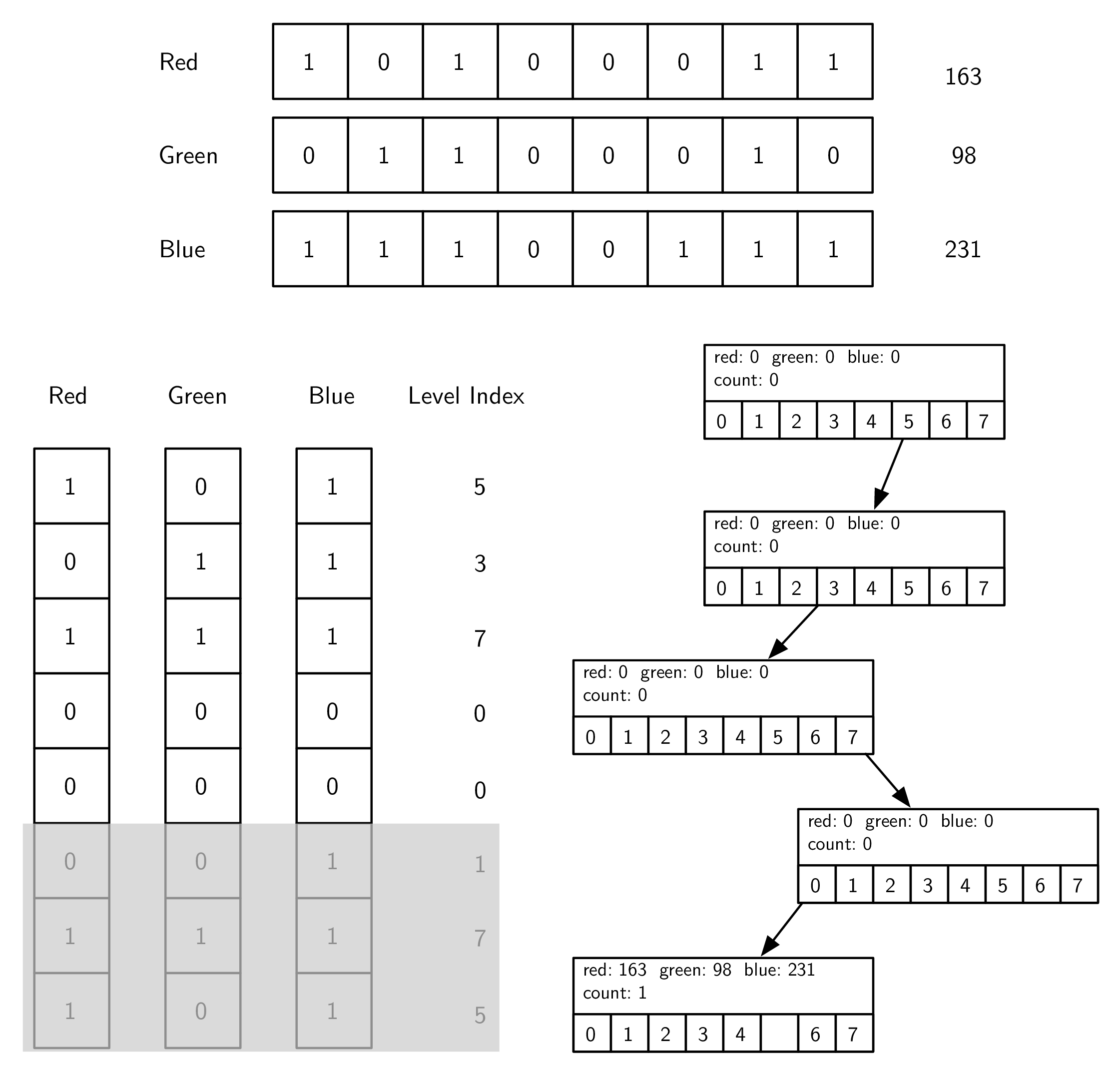
octree we will use the information from the three color components. Figure 11.4.11 shows how we can use the red, green, and blue color values to compute an index for the position of the new node at each level of the tree. The corresponding code for computing the index is on lines 20–26 of Listing 11.4.10.
fun insert(r: Int, g: Int, b: Int, level: Int, outer: Octree) {
    if (level  this.outer!!.maxLevel) {
        val index = computeIndex(r, g, b, level)
        if (this.children[index] == null) {
            this.children[index] = OTNode(this, level + 1, outer)
        }
        this.children[index]!!.insert(r, g, b, level + 1, outer)
    } else {
        if (this.count == 0) {
            this.outer.numLeaves = this.outer.numLeaves + 1
            this.outer.allLeaves.add(this)
        }
        this.red += r
        this.green += g
        this.blue += b
        this.count += 1
    }
}

fun computeIndex(r: Int, g: Int, b: Int, level: Int): Int {
    val nShift = 8 - level
    val rBits = (r shr (nShift - 2)) and 0x04
    val gBits = (g shr (nShift - 1)) and 0x02
    val bBits = (b shr nShift) and 0x01
    return rBits or gBits or bBits
}
The computation of the index combines bits from each of the red, green, and blue color components, starting at the top of the tree with the highest order bits. Figure 11.4.11 shows the binary representation of the red, green, and blue components of 163, 98, 231. At the root of the tree we start with the most significant bit from each of the three color components; in this case the three bits are 1, 0, and 1. Putting these bits together we get binary 101 or decimal 5.
Once we have computed the index appropriate for the current level of the tree, we traverse down into the subtree. In the example in Figure 11.4.11 we follow the link at position 5 in the
children list. If there is no node at position 5, we create one. We keep traversing down the tree until we get to maxLevel. At maxLevel we stop searching and store the data. Notice that we do not overwrite the data in the leaf node, but rather we add the color components to any existing components and increment the reference counter. This allows us to compute the average of any color below the current node in the color cube. In this way, a leaf node in the octree may represent a number of similar colors in the color cube.
The
find method, shown in Listing 11.4.12, uses the same method of index computation as the insert method to traverse the tree in search of a node matching the red, green, and blue components.
find Methodfun find(r: Int, g: Int, b: Int, level: Int): Pixel {
if (level < this.outer!!.maxLevel) {
val index = computeIndex(r, g, b, level)
if (this.children[index] != null) {
return this.children[index]!!.find(r, g, b, level + 1)
} else if (this.count > 0) {
return Pixel(
this.red / this.count,
this.green / this.count, this.blue / this.count
)
} else {
throw Exception("No leaf node to represent RGB($r, $g, $b)")
}
} else {
return Pixel(
this.red / this.count,
this.green / this.count, this.blue / this.count
)
}
}
find needs to return three values, so we use the Pixel data class that we defined above the Octree class.
The
find method has three exit conditions:
-
We have reached the maximum level of the tree and so we return the average of the color information stored in this leaf node (see lines 7–10).
-
We have found a leaf node at a height less than
maxLevel(see lines 4–5). This is possible only after the tree has been reduced. See below. -
We try to follow a path into a nonexistent subtree, which is an error.
The final aspect of the
OTNode class is the merge method. It allows a parent to subsume all of its children and become a leaf node itself. If you remember back to the structure of the octree where each parent cube fully encloses all the cubes represented by the children, you will see why this makes sense. When we merge a group of siblings we are effectively taking a weighted average of the colors represented by each of those siblings. Since all the siblings are relatively close to each other in color space, the average is a good representation of all of them. Figure 11.4.13 illustrates the merge process for some sibling nodes.
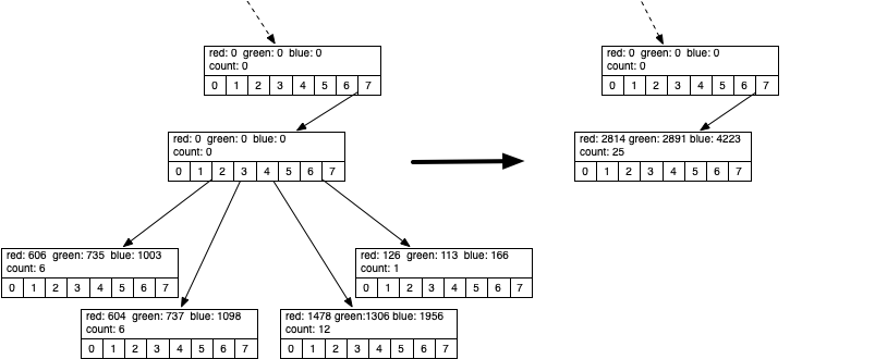
Figure 11.4.13 shows the red, green, and blue components represented by the four leaf nodes whose identifying color values are (101, 122, 167), (100, 122, 183), (123, 108, 163), and (126, 113, 166). As you can see in Listing 11.4.12, the identifying values are calculated by dividing the color values by the count. Notice how close they are in the overall color space. The leaf node that gets created from all of these has an ID of (112, 115, 168). This is close to the average of the four, but weighted more towards the third color tuple due to the fact that it had a reference count of 12.
merge methodfun merge() {
for (child in this.children) {
if (child != null) {
if (child.count > 0) {
val removed = this.outer!!.allLeaves.remove(child)
this.outer.numLeaves -= 1
} else {
println("Recursively merging non-leaf")
child.merge()
}
this.count += child.count
this.red += child.red
this.green += child.green
this.blue += child.blue
}
}
for (i in 0 ..< 8) {
this.children[i] = null
}
}
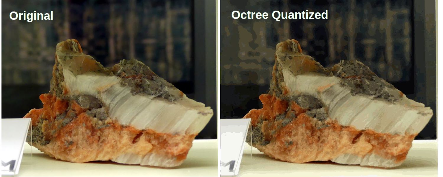
Because the
octree uses only colors that are really present in the image and faithfully preserves colors that are often used, the final quantized image from the octree is much higher quality than the simple method we used to start this section. Figure 11.4.15 shows a comparison of the original image with the quantized image.
There are many additional ways to compress images using techniques such as run-length encoding, discrete cosine transform, and Huffman coding. Any of these algorithms are within your grasp, and we encourage you to look them up and read about them. In addition, quantized images can be improved by using a technique known as dithering. Dithering is a process by which different colors are placed near each other so that the eye blends the colors together, forming a more realistic image. This is an old trick used by newspapers for doing color printing using just black plus three different colors of ink. Again, you can research dithering and try to apply it to some images on your own.
You have attempted of activities on this page.
