Section 10.20 Dijkstra’s Algorithm
The algorithm we are going to use to determine the shortest path is called Dijkstra’s algorithm. Dijkstra’s algorithm is an iterative algorithm that provides us with the shortest path from one particular starting node to all other nodes in the graph. Again this is similar to the results of a breadth-first search.
To keep track of the total cost from the start node to each destination, we will use a map called
distance. This map will contain the current total weight of the smallest weight path from the start to the vertex in question. The algorithm iterates once for every vertex in the graph; however, the order that it iterates over the vertices is controlled by a priority queue. The value that is used to determine the order of the objects in the priority queue is distance. When a vertex is first created, distance is set to a very large number. Specifically, we set it to the largest possible value in Kotlin for a Double. As we have previously seen, in order to manage our data with a priority queue, we need to create a data class holding both the vertex as well as the distance (which will be used as the priority). We need to make that data class Comparable so that the priority queue can do comparisons between items within.
The code for Dijkstra’s algorithm is shown in Listing 10.20.1. When the algorithm finishes, the distances are set correctly as is the
previous map, which indicates predecessor links along the shortest path for each vertex.
class DijkstraSolver<V>(val graph: GraphADT<V>, val start: V) {
    val previous = mutableMapOf<V, V?>()
    val distance = mutableMapOf<V, Double>()

    init {
        dijsktra(start)
    }

    data class PqItem<V>(val vertex: V, val distance: Double):
            Comparable<PqItem<V>> {

        override fun compareTo(other: PqItem<V>): Int {
            return (this.distance - other.distance).toInt()
        }
    }

    private fun dijsktra(start: V) {
        // Initialize distances to all vertices
        for (vertex in graph.getVertices()) {
            distance[vertex] = Double.MAX_VALUE
        }
        distance[start] = 0.0
        previous[start] = null

        // Insert into priority queue
        val pqItems = mutableListOf<PqItem<V>>()
        for (vertex in graph.getVertices()) {
            pqItems.add(PqItem(vertex, distance[vertex]!!))
        }
        val pq = BinaryHeapPriorityQueue(pqItems)

        while (!pq.isEmpty()) {
            val (curV, curDist) = pq.delete()!!
            for (nbrV in graph.getNeighbors(curV)!!) {
                val newDist = curDist + graph.getWeight(curV, nbrV)!!
                if (newDist < distance[nbrV]!!) {
                    val oldDist = distance[nbrV]!!
                    distance[nbrV] = newDist
                    previous[nbrV] = curV

                    // update priority
                    pq.removeElement(PqItem(nbrV, oldDist))
                    pq.insert(PqItem(nbrV, newDist))
                }
            }
        }
    }
}
We have needed to make one update to our priority queue, which is to add a
removeElement method. As you can see in line 42, this method is used when the distance to a vertex that is already in the queue is reduced, and thus the vertex needs to be removed (with the old priority) and re-added with the new one.
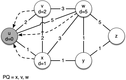
Let’s walk through an application of Dijkstra’s algorithm one vertex at a time using the following sequence of figures as our guide. We begin with the vertex \(u\text{.}\) The three vertices adjacent to \(u\) are \(v, w,\) and \(x\text{.}\) Since the initial distances to \(v, w,\) and \(x\) are all initialized to
Double.MAX_VALUE, the new costs to get to them through the start node are all their direct costs. So we update the costs to each of these three nodes. We also set the predecessor for each node to \(u\) and we add each node to the priority queue. We use the distance as the key for the priority queue. The state of the algorithm is shown in Figure 10.20.2.
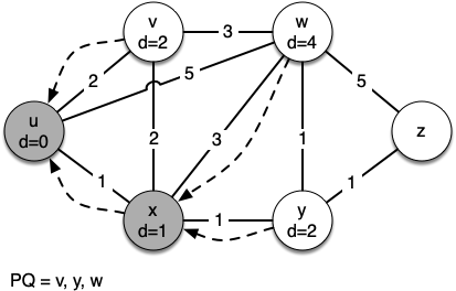
In the next iteration of the
while loop we examine the vertices that are adjacent to \(x\text{.}\) The vertex \(x\) is next because it has the lowest overall cost and therefore bubbled its way to the beginning of the priority queue. At \(x\) we look at its neighbors \(u, v, w,\) and \(y\text{.}\) For each neighboring vertex we check to see if the distance to that vertex through \(x\) is smaller than the previously known distance. Obviously this is the case for \(y\) since its distance was Double.MAX_VALUE. It is not the case for \(u\) or \(v\) since their distances are 0 and 2 respectively. However, we now learn that the distance to \(w\) is smaller if we go through \(x\) than from \(u\) directly to \(w\text{.}\) Since that is the case we update \(w\) with a new distance and change the predecessor for \(w\) from \(u\) to \(x\text{.}\) See Figure 10.20.3 for the state of all the vertices.
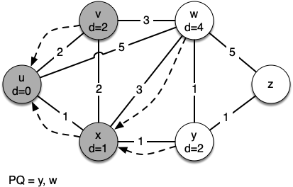
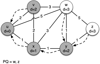
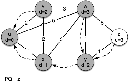
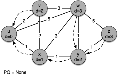
The next step is to look at the vertices neighboring \(v\) (see Figure 10.20.4). This step results in no changes to the graph, so we move on to node \(y\text{.}\) At node \(y\) (see Figure 10.20.5) we discover that it is cheaper to get to both \(w\) and \(z\text{,}\) so we adjust the distances and predecessor links accordingly. Finally we check nodes \(w\) and \(z\) (see Figure 10.20.6 and Figure 10.20.7). However, no additional changes are found and so the priority queue is empty and Dijkstra’s algorithm exits.
It is important to note that Dijkstra’s algorithm works only when the weights are all positive. You should convince yourself that if you introduced a negative weight on one of the edges of the graph in Section 10.19, the algorithm would never exit.
We will note that to route messages through the internet, other algorithms are used for finding the shortest path. One of the problems with using Dijkstra’s algorithm on the internet is that you must have a complete representation of the graph in order for the algorithm to run. The implication of this is that every router has a complete map of all the routers in the internet. In practice this is not the case and other variations of the algorithm allow each router to discover the graph as they go. One such algorithm that you may want to read about is called the distance vector routing algorithm.
You have attempted of activities on this page.
