Section 10.15 General Depth-First Search
The knight’s tour is a special case of a depth-first search where the goal is to create the deepest depth-first tree without any branches. The more general depth-first search is actually easier. Its goal is to search as deeply as possible, connecting as many nodes in the graph as possible and branching where necessary.
It is even possible that a depth-first search will create more than one tree. When the depth-first search algorithm creates a group of trees we call this a depth-first forest. As with the breadth-first search, our depth-first search makes use of predecessor links to construct the tree. In addition, the depth-first search will make use of two additional instance variables, which we will create in our
DfsSolver class. The new instance variables are the discovery and closing times. The discovery time tracks the number of steps in the algorithm before a vertex is first encountered. The closing time is the number of steps in the algorithm before a vertex is complete, meaning that all of its neighbors have been completely explored. As we will see after looking at the algorithm, the discovery and closing times of the nodes provide some interesting properties we can use in later algorithms.
The code for our depth-first search is shown in Listing 10.15.1. As in previous sections, we will use a class to wrap up our code, since we have variables that we need to maintain over multiple method calls (such as
time). Looking at line 13 you will notice that the dfsAll method iterates over all of the vertices in the graph calling dfs on the nodes that have not been worked on yet. The reason we iterate over all the nodes, rather than simply searching from a chosen starting node, is to make sure that all nodes in the graph are considered and that no vertices are left out of the depth-first forest. Iterating over all the vertices in an instance of a graph is a natural thing to do, and in our next two algorithms we will see why keeping track of the depth-first forest is important.
DFSSolver Classclass DfsSolver<V>(val graph: GraphADT<V>) {
val previous = mutableMapOf<V, V?>()
private val visited = mutableSetOf<V>()
private var time = 0 // also referred to as "discovery time"
val closingTime = mutableMapOf<V, Int>()
init {
dfsAll()
}
private fun dfsAll() {
for (vertex in graph.getVertices()) {
previous[vertex] = null
}
for (start in graph.getVertices()) {
if (start !in visited) {
dfs(start)
}
}
}
private fun dfs(vertex: V) {
time += 1
visited.add(vertex)
val neighbors = graph.getNeighbors(vertex)
if (neighbors == null) {
return
}
for (neighbor in neighbors) {
if (neighbor !in visited) {
previous[neighbor] = vertex
dfs(neighbor)
}
}
time += 1
closingTime[vertex] = time
}
}
Aside: A difference with how we implemented BFS.
The
dfs method starts with a single vertex called Vertex and explores all of the neighboring unvisited vertices as deeply as possible. If you look carefully at the code for dfs and compare it to breadth-first search, what you should notice is that the dfsVisit algorithm is similar to bfs, but on the last line of the inner for loop, dfs calls itself recursively to continue the search at a deeper level, whereas bfs adds the node to a queue for later exploration. It is interesting to note that where bfs uses a queue, dfs uses a stack. You don’t see a stack in the code, but it is implicit in the recursive call to dfsVisit.
The following sequence of figures illustrates the depth-first search algorithm in action for a small graph. In these figures, the white nodes are those that have not been visited yet; the gray nodes are the ones in progress, and the black are the ones for whom all paths from that node have been completely explored.
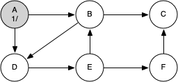
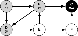
The search begins at vertex A of the graph (Figure 10.15.2). Since all of the vertices are white at the beginning of the search the algorithm visits vertex A. The first step in visiting a vertex is to set the color to gray, which indicates that the vertex is being explored, and the discovery time is set to 1. Since vertex A has two adjacent vertices (B, D) each of those need to be visited as well. We’ll make the arbitrary decision that we will visit the adjacent vertices in alphabetical order.
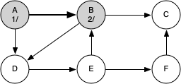
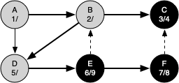
Vertex B is visited next (Figure 10.15.3), so its color is set to gray and its discovery time is set to 2. Vertex B is also adjacent to two other nodes (C, D) so we will follow the alphabetical order and visit node C next.
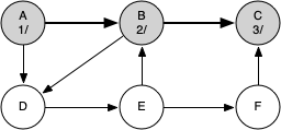
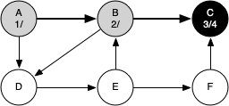
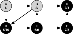
Visiting vertex C (Figure 10.15.4) brings us to the end of one branch of the tree. After coloring the node gray and setting its discovery time to 3, the algorithm also determines that there are no adjacent vertices to C. This means that we are done exploring node C and so we can color the vertex black and set the closing time to 4. You can see the state of our search at this point in Figure 10.15.5.
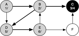
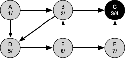
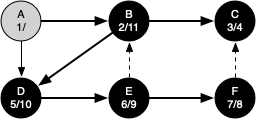
Since vertex C is the end of one branch, we now return to vertex B and continue exploring the nodes adjacent to B. The only additional vertex to explore from B is D, so we can now visit D (Figure 10.15.6) and continue our search from vertex D. Vertex D quickly leads us to vertex E (Figure 10.15.7). Vertex E has two adjacent vertices, B and F. Normally we would explore these adjacent vertices alphabetically, but since B is already colored gray the algorithm recognizes that it should not visit B since doing so would put the algorithm in a loop! So exploration continues with the next vertex in the list, namely F (Figure 10.15.8).
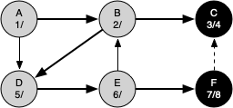
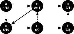
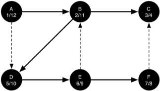
Vertex F has only one adjacent vertex, C, but since C is colored black there is nothing else to explore, and the algorithm has reached the end of another branch. From here on, you will see in Figure 10.15.9 through Figure 10.15.14 that the algorithm works its way back to the first node, setting closing times and coloring vertices black.
The discovery and closing times for each node display a property called the parenthesis property. This property means that all the children of a particular node in the depth-first tree have a later discovery time and an earlier closing time than their parent. Figure 10.15.14 shows the tree constructed by the depth-first search algorithm.
You have attempted of activities on this page.
