Because \(\log {(x)}\) grows very slowly as \(x\) increases from 1, logarithms are useful for modeling phenomena that take on a very wide range of values. For example, biologists study how metabolic functions such as heart rate are related to an animal’s weight, or mass. The table shows the mass in kilograms of several mammals.
Imagine trying to scale the \(x\)-axis to show all of these values. If we set tick marks at intervals of 10,000 kg, as shown below, we can plot the mass of the whale, and maybe the elephant, but the dots for the smaller animals will be indistinguishable. (On this graph, the first dot would have to represent the shrew, cat, wolf and horse!)
On the other hand, we can plot the mass of the cat if we set tick marks at intervals of 1 kg, but the axis will have to be extremely long to include even the wolf. We cannot show the masses of all these animals on the same scale.
To get around this problem, we’ll compute the the log of each mass, and use the logs on a new scale. The table below shows the base 10 log of each animal’s mass, rounded to 2 decimal places.
We’d need to keep in mind that we are plotting the logs of the animals’ masses, and not the actual masses. However, remember that a logarithm is really an exponent! For example, the mass of the horse is 300 kg, and
Compare this new scale to the previous one. It looks almost the same, except that the number line is labeled with powers of 10. Even though we computed the log of each mass, we still plotted the actual mass of each animal, in its form as a power of 10. It is the scale on the number line that has changed.
A scale labeled with powers of 10 is called a logarithmic scale, or log scale. The powers of 10 on a log scale are evenly spaced, so that the actual values at the tick marks look like this.
We can see right away that the increments between tick marks on a log scale are not equal, as they are on a usual linear scale. The increments get larger as we move from left to right on the scale. However, when we are plotting powers of 10 we use the exponents to place the data points on the scale. For example, you can check that the mass of the horse, at \(10^{2.48} = 300\) kg, is plotted about half-way between \(10^2 = 100\) and \(10^3 = 1000\) on the log scale, because 2.48 is about half-way between 2 and 3. Similarly, the mass of the cat, at \(10^{0.60} = 4\) kg, is plotted between \(10^0 = 1\) and \(10^1 = 10\) on the log scale.
Then we plot each number as a power of 10, estimating its position between powers with integer exponents. For example, we plot the first value, \(10^{-3.15}\text{,}\) closer to \(10^{-3}\) than to \(10^{-4}\text{.}\) The finished plot is shown below.
Complete the table by estimating the logarithm of each point plotted on the log scale below. Then use a calculator to give a decimal value for each point.
Log scales allow us to plot a wide range of values, but there is a trade-off. Equal increments on a log scale do not correspond to equal differences in value, as they do on a linear scale. You can see this more clearly if we label the tick marks with their integer values, as well as powers of 10. The difference between \(10^1\) and \(10^0\) is \(10 - 1 = 9\text{,}\) but the difference between \(10^2\) and \(10^1\) is \(100 - 10 = 90\text{.}\)
As we move from left to right on this scale, we multiply the value at the previous tick mark by 10. Moving up by equal increments on a log scale does not add equal amounts to the values plotted; it multiplies the values by equal factors. In the next Example, observe how the integers are plotted on a log scale: they are not evenly spaced.
On the log scale in Example 10.2.4, notice how the integer values are spaced: They get closer together as they approach the next power of \(10\text{.}\) If we would like to label a log scale with integers, we get a very different looking scale, one in which the tick marks are not evenly spaced.
Some applications use log-log graph paper, which scales both axes with logarithmic scales. On the graph in the next Checkpoint, the tick marks between powers of 10 show integer values, as on the scale above.
The opening page of Chapter 6shows the "mouse-to-elephant" curve, a graph of the metabolic rate of mammals as a function of their mass. Here it is again.
You may have already encountered log scales in some everyday applications. In the examples that follow, don’t worry if you aren’t familiar with the science surrounding the application; we will mainly be concerned with the mathematics of using the scale.
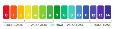
You have probably heard that the pH value of most shampoo is between 7 and 9. The pH scale is a log scale used to measure the acidity of a substance or a chemical compound. Acidity depends on the concentration of hydrogen ions in the substance, denoted by \([H^+]\text{,}\) which can take on a wide range of values, from \(10^{-1}\) to \(10^{-14}\text{.}\)
By taking the log of \([H^+]\) (and changing its sign), we are looking at just its exponent, so that values for pH fall between 0 and 14. A pH value of 7 indicates a neutral solution, and the lower the pH value, the more acidic the substance.
Notice that the pH values are a log scale, so that a decrease of 1 on the pH scale corresponds to an increase in \([H^+]\) by a factor of 10. Thus, lemon juice is 10 times more acidic than vinegar, and battery acid is 100 times more acidic than vinegar.
The decibel scale, used to measure the loudness of a sound, is another example of a logarithmic scale. The loudness of a sound depends on the intensity \(I\) of its sound waves, which is measured in watts per square meter. The decibel value, \(D\text{,}\) is given by
Once again, taking the log of \(I\) simplifies the numbers involved by considering just their exponents. (And dividing by \(10^{-12}\) brings the values into a convenient range.)
Consider the ratio of the intensity of thunder to that of a whisper:
\begin{equation*}
\frac{\text{Intensity of thunder}}{\text{Intensity of a whisper}}
= \frac{10^{-1}}{10^{-10}}= 10^9
\end{equation*}
Thunder is \(10^9\text{,}\) or one billion times more intense than a whisper. It would be impossible to show such a wide range of values on a graph. When we use a log scale, however, there is a difference of only 90 decibels between a whisper and thunder.
Normal breathing generates about \(10^{-11}\) watts per square meter of intensity at a distance of 3 feet. Find the number of decibels for a breath 3 feet away.
From part (a), we know that the sound intensity of breathing is \(10^{-11}\) watts per square meter. We’ll calculate the intensity of conversation from its decibel value.
\begin{align*}
40 \amp = 10 \log_{10}\left(\frac{I}{10^{-12}}\right) \amp\amp\blert{\text{Divide both sides by 10.}}\\
4 \amp = \log_{10}\left(\frac{I}{10^{-12}}\right) \amp\amp\blert{\text{Convert to exponential form.}}\\
\dfrac{I}{10^{-12}} \amp = 10^4 \amp\amp \blert{\text{Multiply both sides by }10^{-12}.}\\
I \amp = 10^4(10^{-12}) = 10^{-8}
\end{align*}
Both the decibel model and the Richter scale in the next example use expressions of the form \(\log\left(\dfrac{a}{b}\right)\text{.}\) Be careful to follow the order of operations when using these models. We must compute the quotient \(\dfrac{a}{b}\) before taking a logarithm. In particular, keep in mind that \(\log\left(\dfrac{a}{b}\right)\) can \(\blert{\text{not}}\) be simplified to \(\dfrac{\log {(a)}}{\log {(b)}}\text{.}\)
One method for measuring the magnitude of an earthquake compares the amplitude \(A\) of its seismographic trace with the amplitude \(A_0\) of the smallest detectable earthquake. The log of their ratio is the Richter magnitude, \(M\text{.}\) Thus,
The Northridge earthquake of January 1994 registered 6.9 on the Richter scale. What would be the magnitude of an earthquake 100 times as powerful as the Northridge quake?
In October 2005, a magnitude 7.6 earthquake struck Pakistan. How much more powerful was this earthquake than the 1989 San Francisco earthquake of magnitude 7.1?
Subsection10.2.6Comparing Quantities on a Log Scale
An earthquake 100, or \(10^2\text{,}\) times as strong is only two units greater in magnitude on the Richter scale. In general, a difference of \(K\) units on the Richter scale (or any logarithmic scale) corresponds to a factor of \(10^K\) units in the intensity of the quake.
A difference of 1.6 on a log scale corresponds to a factor of \(10^{1.6}\) in the actual weights. Thus, the heavier animal is \(10^{1.6}\text{,}\) or 39.8 times as heavy as the lighter animal.
The loudest sound emitted by any living source is made by the blue whale. Its whistles have been measured at 188 decibels and are detectable 500 miles away. Find the intensity of the blue whale’s whistle in watts per square meter.
The probability of discovering an oil field increases with its diameter, defined to be the square root of its area. Use the graph to estimate the diameter of the oil fields at the labeled points, and their probability of discovery. (Source: Deffeyes, 2001)
The order of a stream is a measure of its size. Use the graph to estimate the drainage area, in square miles, for streams of orders 1 through 4. (Source: Leopold, Wolman, and Miller)
The pH of normal rain is 5.6. Some areas of Ontario have experienced acid rain with a pH of 4.5. How many times more acidic is acid rain than normal rain?
At a concert by The Who in 1976, the sound level 50 meters from the stage registered 120 decibels. How many times more intense was this than a 90-decibel sound (the threshold of pain for the human ear)?
A refrigerator produces 50 decibels of noise, and a vacuum cleaner produces 85 decibels. How much more intense are the sound waves from a vacuum cleaner than those from a refrigerator?
In 1964, an earthquake in Alaska measured 8.4 on the Richter scale. An earthquake measuring 4.0 is consideredsmall and causes little damage. How many times stronger was the Alaska quake than one measuring 4.0?
On April 30, 1986, an earthquake in Mexico City measured 7.0 on the Richter scale. On September 21, a second earthquake occurred, this one measuring 8.1, hit Mexico City. How many times stronger was the September quake than the one in April?