Earlier, we used linear regression to fit a line to a collection of data points. In this section we’ll see how to fit a quadratic equation to a collection of data points.
Subsection4.3.1Finding a Quadratic Equation through Three Points
Every linear equation can be written in the form
\begin{equation*}
y=mx+b
\end{equation*}
To find a specific line we must find values for the two parameters (constants) \(m\) and \(b\text{.}\) We need two data points in order to find those two parameters. A quadratic equation, however, has three parameters, \(a,~b,\) and \(c\text{:}\)
\begin{equation*}
y=ax^2+bx+c
\end{equation*}
To find these parameters we need three data points.
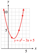
Find values for \(a\text{,}\)\(b\text{,}\) and \(c~\) so that the points \((1, 3)\text{,}\)\((3, 5)\text{,}\) and \((4, 9)\) lie on the graph of \(~y = ax^2 + bx + c\text{.}\)
The simplest way to fit a parabola to a set of data points is to pick three of the points and find the equation of the parabola that passes through those three points.
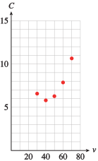
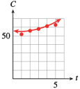
Major Motors Corporation is testing a new car designed for in-town driving. The data below show the cost of driving the car at different speeds. The speeds, \(v\text{,}\) are given in miles per hour, and the cost, \(C\text{,}\) includes fuel and maintenance for driving the car \(100\) miles at that speed.
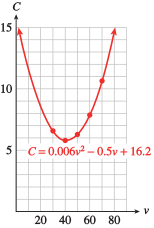
We will use the last three data points, \((50, 6.20)\text{,}\)\((60, 7.80)\text{,}\) and \((70, 10.60)\text{,}\) to fit a parabola to the data. We would like to find the coefficients \(a\text{,}\)\(b\text{,}\) and \(c\) of a parabola \(C = av^2 + bv + c\) that includes the three data points. This gives us a system of equations:
As was the case with linear regression, the graph of the regression equation may not pass through all of the data points, but it should be close to most of them.
According to the model in the previous Example (involving a quadratic model for the cost of driving at different speeds), higher speeds always result in higher driving costs.
Subsection4.3.3Using a Calculator for Quadratic Regression
We can use a graphing calculator or other technology to find an approximate quadratic fit for a set of data. The procedure is similar to the steps for linear regression.
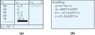
We press STATENTER and enter the data under columns \(L_1\) and \(L_2\text{,}\) as shown below. Next, we calculate the quadratic regression equation and store it in \(Y_1\) by pressing STAT→\(5\)VARS→\(1\)\(1\)ENTER.
The regression equation has the form \(y = ax^2 + bx + c\text{,}\) where \(a = 0.0057\text{,}\)\(b = -0.47\text{,}\) and \(c = 15.56\text{.}\) Notice that \(a\text{,}\)\(b\text{,}\) and \(c\) are all close to the values we computed in Example 4.3.4.
Next, we will graph the data and the regression equation. We press Y= and select Plot1, then press ZOOM\(9\) to see the graph shown below. The parabola seems to pass close to all the data points.
However, try using either the value feature or a table to find the \(y\)-coordinates of points on the regression curve. By comparing these \(y\)-coordinates with our original data points, we find that none of the given data points lies precisely on the parabola.
To test the effects of radiation, a researcher irradiated male mice with various dosages and bred them with unexposed female mice. The table below shows the fraction of fertilized eggs that survived, as a function of the radiation dosage. (Source: Strickberger, Monroe W., 1976)
We must be careful that our data set gives a complete picture of the situation we want to model. A regression equation may fit a particular collection of data and still be a poor model if the rest of the data diverge from the regression graph.
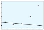
In Example 4.3.4, suppose Major Motors had collected only the first three data points and fit a line through them, as shown at left. This regression line gives poor predictions for the cost of driving at 60 or 70 miles per hour.
Delbert records the height of the tip of the minute hand on the classroom’s clock at different times. The data are shown in the table, where time is measured in minutes since noon. (A negative time indicates a number of minutes before noon.) Find a quadratic regression equation for the data and use it to predict the height of the minute hand’s tip at 40 minutes past noon. Do you believe this prediction is valid?
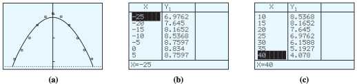
We enter the time data under \(L_1\) and the height data under \(L_2\text{.}\) Then we calculate and store the quadratic regression equation in \(Y_1\text{,}\) as we did in Example 4.3.7. The regression equation is
\begin{equation*}
y = -0.00297x^2 + 0x + 8.834
\end{equation*}
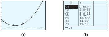
From either the graph of the regression equation or from the table (see figure below), we can see that the fit is not perfect, although the curve certainly fits the data better than any straight line could.
If we scroll down the table, we find that this equation predicts a height of approximately 4.08 feet at time 40 minutes. (See figure (c).) This is a preposterous estimate! The position of the minute hand at 40 minutes after noon should be the same as it was exactly one hour earlier (at 20 minutes before noon), when it was 7.50 feet.
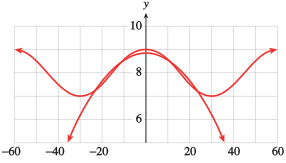
Using the wrong type of function to fit the data is a common error in making predictions. In the Example above, we know that the minute hand of a clock repeats its position every 60 minutes. The graph of the height of its tip oscillates up and down, repeating the same pattern over and over. We cannot describe such a graph using either a linear or a quadratic function.
The graph of the height is shown at left, along with the graph of our quadratic regression equation. You can see that the regression equation fits the actual curve only on a small interval.
Even though your calculator can always compute a regression equation,that equation is not necessarily appropriate for your data. Choosing a reasonable type of regression equation for a particular data set requires knowledge of different kinds of models and the physical or natural laws that govern the situation at hand.
A speeding motorist slams on the brakes when she sees an accident directly ahead of her. The distance she has traveled \(t\) seconds after braking is shown in the table.
Enter the data into your calculator and create a scatterplot. Fit a quadratic regression equation to the data and graph the equation on the scatterplot.
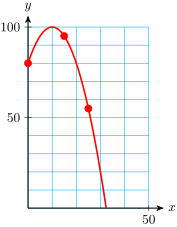
You are in charge of selling tickets to a one-woman show at a local art gallery. Tickets to the opening night were priced at $25, and you sold 30 tickets.
Every night after the opening, you reduce the ticket price by $2. What is the ticket price after \(x\) nights?
Sara plans to start a side business selling eggs. She finds that the total number of eggs produced each day depends on the number of hens confined in the henhouse, as shown in the table.
You are driving at a speed of 60 miles per hour when you step on the brakes. Find a quadratic model for the distance in feet that your car travels in \(t\) seconds after braking. Some data are provided.
In the 1990’s, an outbreak of mad cow disease (Creutzfeldt-Jakob disease) alarmed health officials in England. The table shows the number of deaths each year from the disease.
The Health Protection Agency determined that a quadratic model was the best-fitting model for the data. Find a quadratic regression equation for the data.
Some comets move about the sun in parabolic orbits. In 1973 the comet Kohoutek passed within 0.14 AU (astronomical units), or 21 million kilometers of the sun. Imagine a coordinate system superimposed on a diagram of the comet’s orbit, with the sun at the origin, as shown below. The units on each axis are measured in AU.
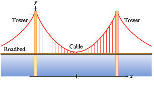
The Akashi Kaikyo bridge in Japan is the longest suspension bridge in the world, with a main span of 1991 meters. Its main towers are 297 meters tall. The roadbed of the bridge is 14 meters thick and clears the water below by 65 meters. The cables on a suspension bridge hang in the shape of parabolas. Imagine a coordinate system superimposed on the diagram of the bridge, as shown in the figure.