8.2. Python Lists Revisited

In Chapter [analysis] we introduced some Big-O performance limits on Python’s list data type. However, we did not yet have the knowledge necessary to understand how Python implements its list data type. in Chapter [basic-data-structures] you learned how to implement a linked list using the nodes and references pattern. However, the nodes and references implementation still did not match the performance of the Python list. In this section we will look at the principles behind the Python list implementation. It is important to recognize that this implementation is not going to be the same as Python’s since the real Python list is implemented in the C programming language. The idea in this section is to use Python to demonstrate the key ideas, not to replace the C implementation.

The key to Python’s implementation of a list is to use a data type called an array common to C, C++, Java, and many other programming languages. The array is very simple and is only capable of storing one kind of data. For example, you could have an array of integers or an array of floating point numbers, but you cannot mix the two in a single array. The array only supports two operations: indexing and assignment to an array index.

The best way to think about an array is that it is one continuous block of bytes in the computer’s memory. This block is divided up into $n$-byte chunks where $n$ is based on the data type that is stored in the array. Figure 1 illustrates the idea of an array that is sized to hold six floating point values.

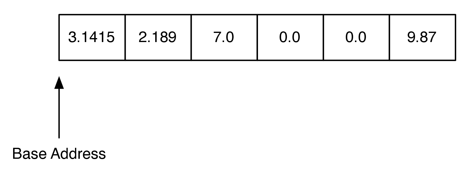
An Array of Floating Point Numbers

In Python, each floating point number uses 16 [1] bytes of memory. So the array in Figure 1 uses a total of 96 [2] bytes. The base address is the location in memory where the array starts. You have seen addresses before in Python for different objects that you have defined. For example: <__main__.Foo object at 0x5eca30> shows that the object Foo is stored at memory address 0x5eca30. The address is very important because an array implements the index operator using a very simple calculation:

item_address = base_address + index * size_of_object

For example, suppose that our array starts at location 0x000040, which is 64 in decimal. To calculate the location of the object at position 4 in the array we simply do the arithmetic: $64+4\cdot 8=96$. Clearly this kind of calculation is $O(1)$. Of course this comes with some risks. First, since the size of an array is fixed, one cannot just add things on to the end of the array indefinitely without some serious consequences. Second, in some languages, like C, the bounds of the array are not even checked, so even though your array has only six elements in it, assigning a value to index 7 will not result in a runtime error. As you might imagine this can cause big problems that are hard to track down. In the Linux operating system, accessing a value that is beyond the boundaries of an array will often produce the rather uninformative error message “segmentation violation.”

The general strategy that Python uses to implement a linked list using an array is as follows:

• Python uses an array that holds references (called pointers in C) to other objects.

• Python uses a strategy called over-allocation to allocate an array with space for more objects than is needed initially.

• When the initial array is finally filled up, a new, bigger array is over-allocated and the contents of the old array are copied to the new array.

The implications of this strategy are pretty amazing. Let’s look at what they are first before we dive into the implementation or prove anything.

• Accessing an itema at a specific location is $O(1)$.

• Appending to the list is $O(1)$ on average, but $O(n)$ in the worst case.

• Popping from the end of the list is $O(1)$.

• Deleting an item from the list is $O(n)$.

• Inserting an item into an arbitrary position is $O(n)$.

Let’s look at how the strategy outlined above works for a very simple implementation. To begin, we will only implement the constructor, a __resize method, and the append method. We will call this class ArrayList. In the constructor we will need to initialize two instance variables. The first will keep track of the size of the current array; we will call this max_size. The second instance variable will keep track of the current end of the list; we will call this one last_index. Since Python does not have an array data type, we will use a list to simulate an array. Listing [lst_arraylistinit] contains the code for the first three methods of ArrayList. Notice that the constructor method initializes the two instance variables described above and then creates a zero element array called my_array. The constructor also creates an instance variable called size_exponent. We will understand how this variable is used shortly.

class ArrayList:
    def __init__(self):
        self.size_exponent = 0
        self.max_size = 0
        self.last_index = 0
        self.my_array = []

    def append(self, val):
        if self.last_index > self.max_size - 1:  |\label{line:lst_arr_size}|
            self.__resize()
        self.my_array[self.last_index] = val
        self.last_index += 1

    def __resize(self):
        new_size = 2 ** self.size_exponent
        print("new_size = ", new_size)
        new_array = [0] * new_size
        for i in range(self.max_size):  |\label{line:lst_arr_cop1}|
            new_array[i] = self.my_array[i]

        self.max_size = new_size
        self.my_array = new_array
        self.size_exponent += 1

Next, we will implement the append method. The first thing append does is test for the condition where last_index is greater than the number of available index positions in the array (line [line:lst_arr_size]). If this is the case then __resize is called. Notice that we are using the double underscore convention to make the resize method private. Once the array is resized the new value is added to the list at last_index, and last_index is incremented by one.

The resize method calculates a new size for the array using $2^{size\mathrm{\_}exponent}$. There are many methods that could be used for resizing the array. Some implementations double the size of the array every time as we do here, some use a multiplier of 1.5, and some use powers of two. Python uses a multiplier of 1.125 plus a constant. The Python developers designed this strategy as a good tradeoff for computers of varying CPU and memory speeds. The Python strategy leads to a sequence of array sizes of $0,4,8,16,24,32,40,52,64,76\dots$ . Doubling the array size leads to a bit more wasted space at any one time, but is much easier to analyze. Once a new array has been allocated, the values from the old list must be copied into the new array; this is done in the loop starting on line [line:lst_arr_cop1]. Finally the values max_size and last_index must be updated, size_exponent must be incremented, and new_array is saved as self.my_array. In a language like C the old block of memory referenced by self.my_array would be explicitly returned to the system for reuse. However, recall that in Python objects that are no longer referenced are automatically cleaned up by the garbage collection algorithm.

Before we move on let’s analyze why this strategy gives us an average $O(1)$ performance for append. The key is to notice that most of the time the cost to append an item $c_i$ is 1. The only time that the operation is more expensive is when last_index is a power of 2. When last_index is a power of 2 then the cost to append an item is $O(last\mathrm{\_}index)$. We can summarize the cost to insert the $i_{th}$ item as follows:

$$\begin{array}{r}{c}_i=\{\begin{array}{l}i\text{ if }i\text{ is a power of 2}\\ 1\text{ otherwise}\end{array}\end{array}$$

Since the expensive cost of copying last_index items occurs relatively infrequently we spread the cost out, or amortize, the cost of insertion over all of the appends. When we do this the cost of any one insertion averages out to $O(1)$. For example, consider the case where you have already appended four items. Each of these four appends costs you just one operation to store in the array that was already allocated to hold four items. When the fifth item is added a new array of size 8 is allocated and the four old items are copied. But now you have room in the array for four additional low cost appends. Mathematically we can show this as follows:

$$\begin{array}{r}\begin{array}{rl}cos{t}_{total}& =n+\sum _{j=0}^{{\log }_{2}n}{2}^j\\ & =n+2n\\ & =3n\end{array}\end{array}$$

The summation in the previous equation may not be obvious to you, so let’s think about that a bit more. The sum goes from zero to ${\log }_{2}n$. The upper bound on the summation tells us how many times we need to double the size of the array. The term $2^j$ accounts for the copies that we need to do when the array is doubled. Since the total cost to append n items is $3n$, the cost for a single item is $3n/n=3$. Because the cost is a constant we say that it is $O(1)$. This kind of analysis is called amortized analysis and is very useful in analyzing more advanced algorithms.

Next, let us turn to the index operators. Listing [lst_arrindex] shows our Python implementation for index and assignment to an array location. Recall that we discussed above that the calculation required to find the memory location of the $i_{th}$ item in an array is a simple $O(1)$ arithmetic expression. Even languages like C hide that calculation behind a nice array index operator, so in this case the C and the Python look very much the same. In fact, in Python it is very difficult to get the actual memory location of an object for use in a calculation like this so we will just rely on list’s built-in index operator. To confirm this, you can always get the Python source code and look at the file listobject.c.

def __getitem__(self, idx):
    if idx < self.last_index:
        return self.my_array[idx]
    raise LookupError("index out of bounds")

def __setitem__(self, idx, val):
    if idx < self.last_index:
        self.my_array[idx] = val
    raise LookupError("index out of bounds")

Finally, let’s take a look at one of the more expensive list operations, insertion. When we insert an item into an ArrayList we will need to first shift everything in the list at the insertion point and beyond ahead by one index position in order to make room for the item we are inserting. The process is illustrated in Figure 2.

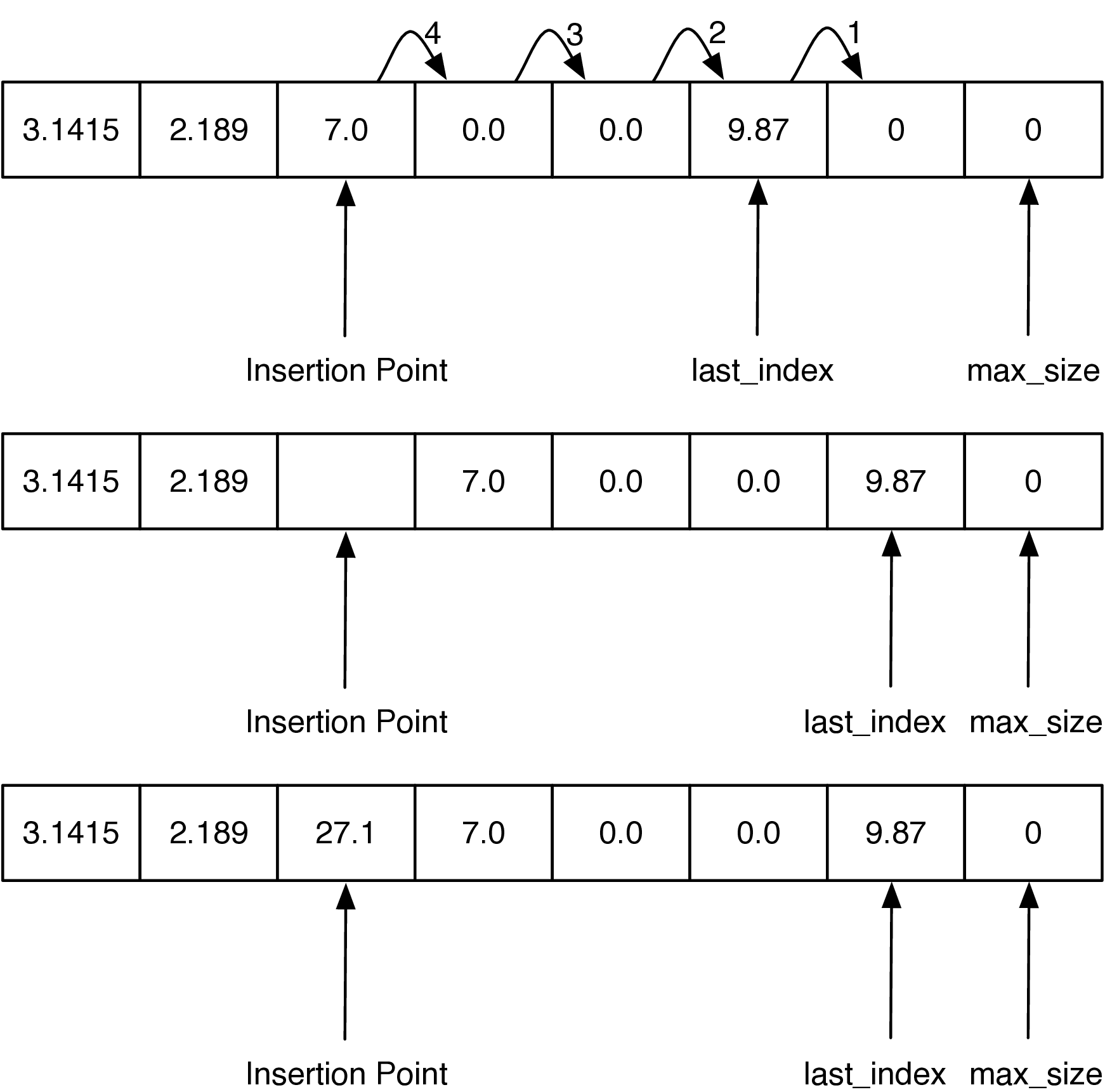
Inserting 27.1 at Index 2 in an ArrayList

The key to implementing insert correctly is to realize that as you are shifting values in the array you do not want to overwrite any important data. The way to do this is to work from the end of the list back toward the insertion point, copying data forward. Our implementation of insert is shown in Listing [lst_arrlistins]. Note how the range is set up on line [line:lst_arrlistins_range] to ensure that we are copying existing data into the unused part of the array first, and then subsequent values are copied over old values that have already been shifted. If the loop had started at the insertion point and copied that value to the next larger index position in the array, the old value would have been lost forever.

def insert(self, idx, val):
    if self.last_index > self.max_size - 1:
        self.__resize()
    for i in range(self.last_index, idx - 1, -1):  |\label{line:lst_arrlistins_range}|
        self.my_array[i + 1] = self.my_array[i]
    self.last_index += 1
    self.my_array[idx] = val

The performance of the insert is $O(n)$ since in the worst case we want to insert something at index 0 and we have to shift the entire array forward by one. On average we will only need to shift half of the array, but this is still $O(n)$. You may want to go back to Chapter [basicds] and remind yourself how all of these list operations are done using nodes and references. Neither implementation is right or wrong; they just have different performance guarantees that may be better or worse depending on the kind of application you are writing. In particular, do you intend to add items to the beginning of the list most often, or does your application add items to the end of the list? Will you be deleting items from the list or only adding new items to the list?

There are several other interesting operations that we have not yet implemented for our ArrayList including: pop, del, index, and making the ArrayList iterable. We leave these enhancements to the ArrayList as an exercise for you.

[1]

8 bytes reference count + 8 bytes pointer to the type object + 8 bytes of data = 24

[2]

sys.getsizeof([3.1415, 2.189, 0.0, 0.0, 9.87]) is 104

You have attempted 1 of 1 activities on this page