Section 9.13 Implementing Knight’s Tour
The search algorithm we will use to solve the knight’s tour problem is called depth first search (DFS). Whereas the breadth first search algorithm discussed in the previous section builds a search tree one level at a time, a depth first search creates a search tree by exploring one branch of the tree as deeply as possible. In this section we will look at two algorithms that implement a depth first search. The first algorithm we will look at directly solves the knight’s tour problem by explicitly forbidding a node to be visited more than once. The second implementation is more general, but allows nodes to be visited more than once as the tree is constructed. The second version is used in subsequent sections to develop additional graph algorithms.
The depth first exploration of the graph is exactly what we need in order to find a path that has exactly 63 edges. We will see that when the depth first search algorithm finds a dead end (a place in the graph where there are no more moves possible) it backs up the tree to the next deepest vertex that allows it to make a legal move.
The
knightTour function takes four parameters: n, the current depth in the search tree; path, a list of vertices visited up to this point; u, the vertex in the graph we wish to explore; and limit the number of nodes in the path. The knightTour function is recursive. When the knightTour function is called, it first checks the base case condition. If we have a path that contains 64 vertices, we return from knightTour with a status of True, indicating that we have found a successful tour. If the path is not long enough we continue to explore one level deeper by choosing a new vertex to explore and calling knightTour recursively for that vertex.
DFS also uses colors to keep track of which vertices in the graph have been visited. Unvisited vertices are colored white, and visited vertices are colored gray. If all neighbors of a particular vertex have been explored and we have not yet reached our goal length of 64 vertices, we have reached a dead end. When we reach a dead end we must backtrack. Backtracking happens when we return from
knightTour with a status of False. In the breadth first search we used a queue to keep track of which vertex to visit next. Since depth first search is recursive, we are implicitly using a stack to help us with our backtracking. When we return from a call to knightTour with a status of False, in line 11, we remain inside the while loop and look at the next vertex in nbrList.
Listing 3
from pythonds.graphs import Graph, Vertex
def knightTour(n,path,u,limit):
        u.setColor('gray')
        path.append(u)
        if n < limit:
            nbrList = list(u.getConnections())
            i = 0
            done = False
            while i < len(nbrList) and not done:
                if nbrList[i].getColor() == 'white':
                    done = knightTour(n+1, path, nbrList[i], limit)
                i = i + 1
            if not done:  # prepare to backtrack
                path.pop()
                u.setColor('white')
        else:
            done = True
        return done
Let’s look at a simple example of
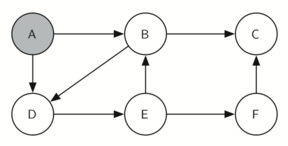
knightTour in action. You can refer to the figures below to follow the steps of the search. For this example we will assume that the call to the getConnections method on line 6 orders the nodes in alphabetical order. We begin by calling knightTour(0,path,A,6).
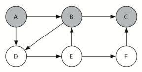
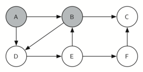
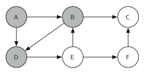
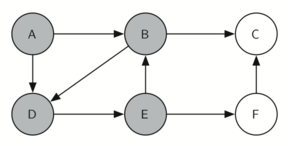
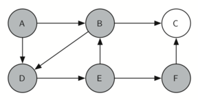
knightTour starts with node A Figure 9.13.1. The nodes adjacent to A are B and D. Since B is before D alphabetically, DFS selects B to expand next as shown in Figure 9.13.2. Exploring B happens when knightTour is called recursively. B is adjacent to C and D, so knightTour elects to explore C next. However, as you can see in Figure 9.13.3 node C is a dead end with no adjacent white nodes. At this point we change the color of node C back to white. The call to knightTour returns a value of False. The return from the recursive call effectively backtracks the search to vertex B (see Figure 9.13.4). The next vertex on the list to explore is vertex D, so knightTour makes a recursive call moving to node D (see Figure 9.13.5). From vertex D on, knightTour can continue to make recursive calls until we get to node C again (see Figure 9.13.6, Figure 9.13.7, and Figure 9.13.8). However, this time when we get to node C the test n < limit fails so we know that we have exhausted all the nodes in the graph. At this point we can return True to indicate that we have made a successful tour of the graph. When we return the list, path has the values [A,B,D,E,F,C], which is the the order we need to traverse the graph to visit each node exactly once.
Graph with node ’fool’ as the central node connected to four adjacent nodes labeled ’pool’, ’foil’, ’foul’, and ’cool’, each marked with the number ’1’. Below the graph is a visual representation of a queue with the nodes ’pool’, ’foil’, ’foul’, and ’cool’ lined up in order.

Graph with nodes A, B, C, D, E, and F, with node B highlighted, indicating exploration from node B to nodes A and E.
Graph highlighting node C, showing no further connections, indicating that C is a dead end in the search process.
Graph with a backtrack path from node C to node B, illustrating the step of returning to node B to continue the search.
Graph with node D highlighted, indicating the exploration is continuing from node D to nodes A and E.
Graph focusing on node E, with exploration proceeding from node E to nodes B and D.
Graph with node F highlighted, representing the search exploring potential paths from node F to node C.
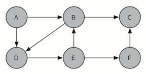
Final graph with all nodes no longer highlighted, representing the completion of the depth-first search process.
Figure 9.13.9 shows you what a complete tour around an eight-by-eight board looks like. There are many possible tours; some are symmetric. With some modification you can make circular tours that start and end at the same square.
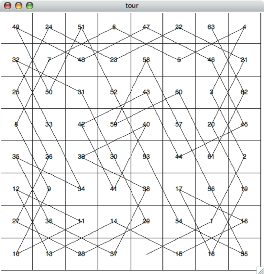
Image depicting a graph overlaid on an 8x8 chessboard grid representing a complete Knight’s Tour. The nodes, numbered from 0 to 63, correspond to the squares of the chessboard. Lines crisscross the grid, mapping the knight’s moves in a sequential path that visits each square exactly once. The complex web of lines indicates the knight’s route, creating a Hamiltonian circuit where the start and end points are connected. Captioned ’Figure 11: A Complete Tour of the Board’.
Reading Questions Reading Questions
2.
You have attempted 1 of 3 activities on this page.
