10.5. Heavy-Tailed Distributions
If the sand pile model is in a critical state, we expect to find heavy-tailed distributions for quantities like the duration and size of avalanches. So let’s take a look.
We’ll make a larger sand pile, with n=50 and an initial level of 30, and run until equilibrium:
pile2 = SandPile(n=50, level=30)
pile2.run()
Next, let’s run 100,000 random drops:
iters = 100000
res = [pile2.drop_and_run() for _ in range(iters)]
As the name suggests, drop_and_run calls drop and run and returns the duration of the avalanche and total number of cells that toppled.
So res is a list of (T, S) tuples, where T is duration, in time steps, and S is cells toppled. We can use np.transpose to unpack res into two NumPy arrays:
T, S = np.transpose(res)
A large majority of drops have duration 1 and no toppled cells; if we filter them out before plotting, we get a clearer view of the rest of the distribution.
T = T[T>1]
S = S[S>0]
The distributions of T and S have many small values and a few very large ones. We will use the Pmf class to make a PMF of the values, that is, a map from each value to its probability of occurring (see Section 6.4).
pmfT = Pmf(T)
pmfS = Pmf(S)

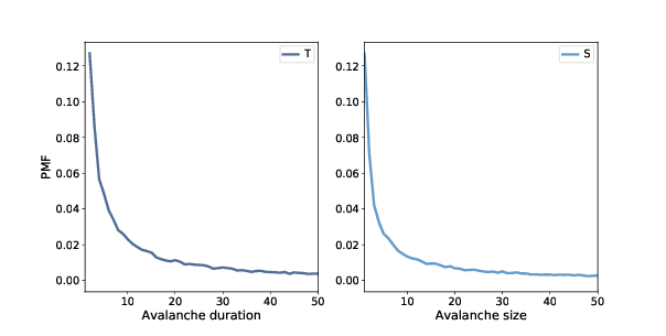
Figure 10.2: Distribution of avalanche duration (left) and size (right), linear scale.

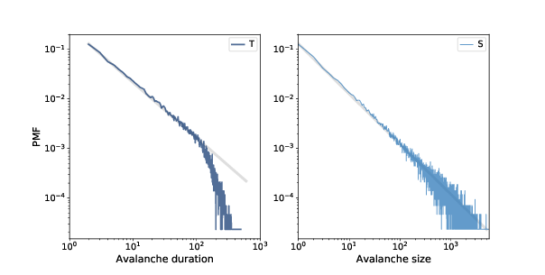
Figure 10.3: Distribution of avalanche duration (left) and size (right), log-log scale.
Figure 10.2 shows the results for values less than 50.
As we saw in Section 6.5, we can get a clearer picture of these distributions by plotting them on a log-log scale, as shown in Figure 10.3.
For values between 1 and 100, the distributions are nearly straight on a log-log scale, which is characteristic of a heavy tail. The gray lines in the figure have slopes near -1, which suggests that these distributions follow a power law with parameters near \(α=1\).
For values greater than 100, the distributions fall away more quickly than the power law model, which means there are fewer very large values than the model predicts. One possibility is that this effect is due to the finite size of the sand pile; if so, we might expect larger piles to fit the power law better.
Another possibility, which you can explore in one of the exercises at the end of this chapter, is that these distributions do not strictly obey a power law. But even if they are not power-law distributions, they might still be heavy-tailed.
-
Q-1:
- For values between 1 and 100
- The distributions are nearly straight on a log-log scale, which is characteristic of a heavy tail.
- For values greater than 100
- The distributions fall away more quickly than the power law model, which means there are fewer very large values than the model predicts.