6.8. Cumulative Distributions

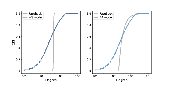
Figure 6.4: CDF of degree in the Facebook dataset along with the WS model (left) and the BA model (right), on a log-x scale.
Figure 6.4 represents the degree distribution by plotting the probability mass function (PMF) on a log-log scale. That’s how Barabási and Albert present their results and it is the representation used most often in articles about power law distributions. But it is not the best way to look at data like this.
A better alternative is a cumulative distribution function (CDF), which maps from a value, x, to the fraction of values less than or equal to x.
Given a Pmf, the simplest way to compute a cumulative probability is to add up the probabilities for values up to and including x:
def cumulative_prob(pmf, x):
ps = [pmf[value] for value in pmf if value<=x]
return np.sum(ps)
For example, given the degree distribution in the dataset, pmf_fb, we can compute the fraction of users with 25 or fewer friends:
>>> cumulative_prob(pmf_fb, 25)
0.506
The result is close to 0.5, which means that the median number of friends is about 25.
CDFs are better for visualization because they are less noisy than PMFs. Once you get used to interpreting CDFs, they provide a clearer picture of the shape of a distribution than PMFs.
The thinkstats module provides a class called Cdf that represents a cumulative distribution function. We can use it to compute the CDF of degree in the dataset.
from thinkstats2 import Cdf
cdf_fb = Cdf(degrees(fb), label='Facebook')
And thinkplot provides a function called Cdf that plots cumulative distribution functions.
thinkplot.Cdf(cdf_fb)
Figure 6.4 shows the degree CDF for the Facebook dataset along with the WS model (left) and the BA model (right). The x-axis is on a log scale.

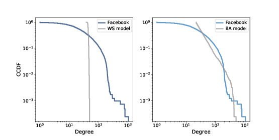
Figure 6.5: Complementary CDF of degree in the Facebook dataset along with the WS model (left) and the BA model (right), on a log-log scale.
Clearly the CDF for the WS model is very different from the CDF from the data. The BA model is better, but still not very good, especially for small values.
In the tail of the distribution (values greater than 100) it looks like the BA model matches the dataset well enough, but it is hard to see. We can get a clearer view with one other view of the data: plotting the complementary CDF on a log-log scale.
The complementary CDF (CCDF) is defined
This definition is useful because if the PMF follows a power law, the CCDF also follows a power law:
where \(x_m\) is the minimum possible value and \(α\) is a parameter that determines the shape of the distribution.
Taking the log of both sides yields:
So if the distribution obeys a power law, we expect the CCDF on a log-log scale to be a straight line with slope −α.
Figure 6.5 shows the CCDF of degree for the Facebook data, along with the WS model (left) and the BA model (right), on a log-log scale.
With this way of looking at the data, we can see that the BA model matches the tail of the distribution (values above 20) reasonably well. The WS model does not.