6.6. Barabási-Albert Model

In 1999 Barabási and Albert published a paper, “Emergence of Scaling in Random Networks”, that characterizes the structure of several real-world networks, including graphs that represent the interconnectivity of movie actors, web pages, and elements in the electrical power grid in the western United States.

They measure the degree of each node and compute PMF(k), the probability that a vertex has degree k. Then they plot PMF(k) versus k on a log-log scale. The plots fit a straight line, at least for large values of k, so Barabási and Albert conclude that these distributions are heavy-tailed.

They also propose a model that generates graphs with the same property. The essential features of the model, which distinguish it from the WS model, are:

Growth: Instead of starting with a fixed number of vertices, the BA model starts with a small graph and adds vertices one at a time.

Preferential attachment: When a new edge is created, it is more likely to connect to a vertex that already has a large number of edges. This “rich get richer” effect is characteristic of the growth patterns of some real-world networks.

Finally, they show that graphs generated by the Barabási-Albert (BA) model have a degree distribution that obeys a power law.

Graphs with this property are sometimes called scale-free networks, for reasons we won’t explain right now.

NetworkX provides a function that generates BA graphs. We will use it first; then we’ll see how it works.

ba = nx.barabasi_albert_graph(n=4039, k=22)

The parameters are n, the number of nodes to generate, and k, the number of edges each node starts with when it is added to the graph. We chose k=22 because that is the average number of edges per node in the dataset.

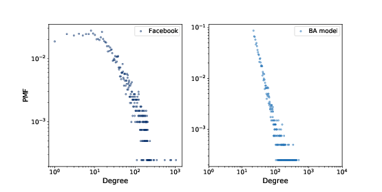
Figure 6.3: PMF of degree in the Facebook dataset and in the BA model, on a log-log scale.

The resulting graph has $4039$ nodes and $21.9$ edges per node. Since every edge is connected to two nodes, the average degree is $43.8$, very close to the average degree in the dataset, $43.7$.

And the standard deviation of degree is $40.9$, which is a bit less than in the dataset, $52.4$, but it is much better than what we got from the WS graph, $1.5$.

Figure 6.3 shows the degree distributions for the Facebook dataset and the BA model on a log-log scale. The model is not perfect; in particular, it deviates from the data when k is less than $10$. But the tail looks like a straight line, which suggests that this process generates degree distributions that follow a power law.

So the BA model is better than the WS model at reproducing the degree distribution. But does it have the small world property?

In this example, the average path length, L, is $2.5$, which is even more “small world” than the actual network, which has L=3.69. So that’s good, although maybe too good.

On the other hand, the clustering coefficient, C, is $0.037$, not even close to the value in the dataset, $0.61$. So that’s a problem.

Table 6.1 summarizes these results. The WS model captures the small world characteristics, but not the degree distribution. The BA model captures the degree distribution, at least approximately, and the average path length, but not the clustering coefficient.

In the exercises at the end of this chapter, you can explore other models intended to capture all of these characteristics.

Table 6.1: Characteristics of the Facebook dataset compared to two models.

You have attempted 1 of 2 activities on this page