What Is A Formula?
Formulas are a way of manipulating data in Sheets. A formula processes data in the same way a calculator does, but in a more organized and useful way that allows you to combine calculations.
All formulas start with the = character. This tells Sheets that this cell is
a formula, rather than raw data. What makes formulas so useful is that the input
to a formula can be new data (e.g. =1+1), or existing data from cells (e.g.
=A1+A2), or a combination (e.g. =A1+1). Below are some illustrative
examples of how formulas work.
Note that if Sheets cannot parse or calculate your formula, you will see an error. See this section for more on errors.
Example: Chocolate Cake
Suppose you are going to a party, and you decide to bake a cake. Your favorite is chocolate cake, so you decide to make this “quick chocolate cake”. You note that the recipe serves 12, so you ask the party hosts how many guests are attending. They say they will need 18 servings.
Since you are now more familiar with Sheets, instead of manually calculating, for each ingredient, how to alter this recipe for 18 people, you use a formula. Sheets allows you to perform the same calculation for all ingredients, with one formula.
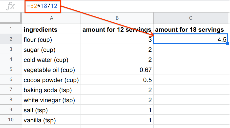
First, you enter the recipe for 12 servings into a table. (Note that for the
ingredients with fractional amounts like 2/3 cup vegetable oil, you need to use
a formula, namely =2/3).
Now, you know that for 18 people, you will need to scale up everything to 18. You can do this by multiplying each ingredient by the scale factor of 18/12. (You can think of this as dividing by 12 to get the amounts for 1 serving, then multiplying by 18 to get the amounts for 18 servings.)
You can use column C to write a formula to get the amounts for 18 servings. First, you need to write the formula for row 2, namely flour. The amount for 12 servings is in cell B2. You want to upsize this ingredient by a factor of 18/12, so the formula is as follows.
=B2*18/12

So for 18 servings, you need 4.5 cups of flour. Now, it’s as simple as copy-pasting this same formula to the other rows. You can do this using in-built copy-paste functionality, or you can drag down from the corner of the cell.
The best thing about Sheets is that you could recreate this recipe no matter how the numbers change. For example, suppose the hosts ask you to bring enough for 23.771 servings. (There are 24 people, but one person is on a diet, and has asked for only 0.771 servings.) You can actually encode the number of servings into the formula, so that the shopping list automatically updates whenever you update the number of servings.
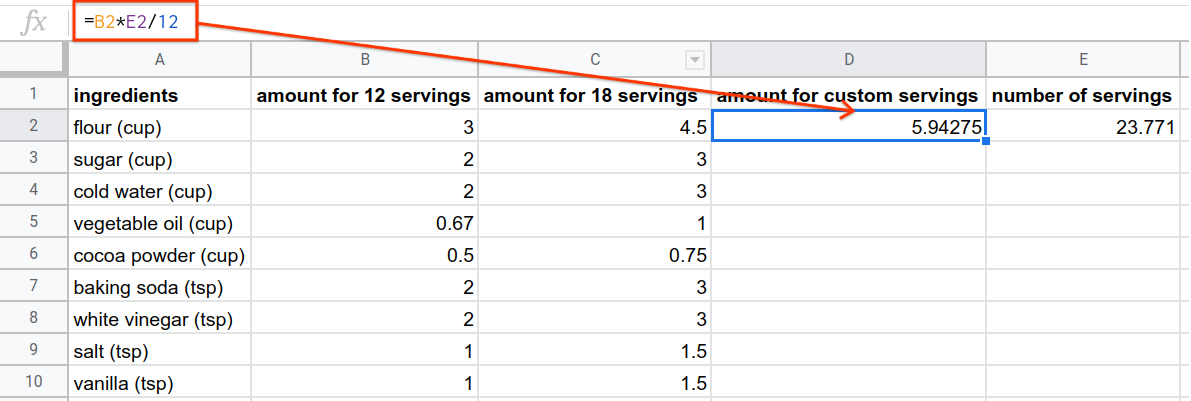
Use column D to show the amount required for the custom number of servings, and use cell E2 to store the desired number of servings, as below.

Now, you can write a formula in column D, similar to the formulas in column C, except instead of hardcoding (entering a number manually) the number of servings, use cell E2 to indicate the number of servings.

Q-6: What do you think will happen if you drag this formula to the rows below?
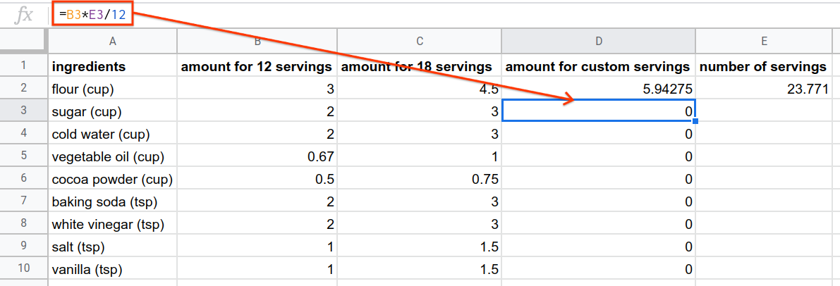
As was done in column C to calculate the recipe amounts for 18 servings, try dragging the formula in column D down to the rows below. You should observe that in this case, copy-pasting the formula did not behave as you might have wanted it to.
Q-7: Why do you think copy-pasting this formula produced all zeros?
The formula in cell D2 references cells B2 and E2. When you copy-paste this formula to D3, Sheets assumes you want the formula to update to reference cells B3 and E3.

This is called relative referencing, because cell referencing in the formula is relative to where the formula is used. (So when it is used in D3, it references B3 and E3.) If you want a cell reference to not update when the formula is copy-pasted, you need to use absolute referencing.
Sheets assumes references are relative. To tell Sheets to reference a cell
absolutely, you need to use the $ symbol.
Consider the cell A1 used in a formula:
If you use A1 in a formula, this is an implicit relative reference. Any cell you copy the formula in will reference a different cell.
If you use $A$1 in a formula, this is an absolute reference. Any cell you copy the formula in will still reference $A$1.
You might be wondering what happens if you only include one of the $ symbols
when referencing A1. This is called semi-absolute referencing, and can be used
to keep the row or column as an absolute reference while using the other as a
relative reference. You can learn more about cell referencing here.
As an example, suppose you have the following sheet.
Q-9: Copy this data to a spreadsheet, and in cell B1, enter the formula
=A1*$A$2. When you copy-paste this formula down, what numbers do you
expect to see?
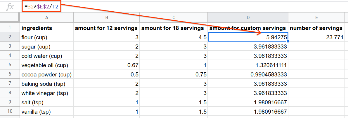
In this chocolate cake example, you want column B to be referenced relatively (so when you copy-paste to rows below, it updates itself), but cell E2 to be referenced absolutely. So, the formula for cell D3 should be as below.
=B2*$E$2/12
Copy-pasting this formula down for the other ingredients now works as intended.

Now, if you update the number of servings you need in cell E2, the amounts for the shopping list magically update themselves.
Doing all of these steps manually, for each ingredient, would be challenging and may result in miscalculations. Doing it in Sheets might take some getting used to, but once you have the hang of using formulas, it makes calculations like this extremely simple!
Example: The Fibonacci Sequence
While it is sometimes useful to use formulas as a type of calculator, formulas are most powerful when extending the same operation to multiple rows or columns. To illustrate this, consider the Fibonacci Sequence.
The Fibonacci Sequence is a sequence of positive numbers where each number is the sum of the previous two numbers in the sequence. The sequence starts with the numbers 0, 1, 1, 2, and goes on infinitely. The sequence looks like:
0, 1, 1, 2, 3, 5, 8, 13, 21, ...
The Fibonacci sequence has a very special and fundamental relationship with nature and art. It can predict, for example, the number of rabbits in a population. Fibonacci numbers also appear in flower and leaf growth. The real-life examples of the Fibonacci sequence don’t stop there. As the numbers in the Fibonacci sequence get larger and larger, the ratio between consecutive numbers in the sequence gets closer and closer to the golden ratio. This number is prevalent in pure mathematics, physics, nature, sculpture, architecture, and art (for example in the Mona Lisa). You can read more about the golden ratio’s appearance in classical and modern art here.
Now, suppose you wanted to generate the 50th number of the Fibonacci sequence. You could do this by hand with lots of mental arithmetic, but this would take a long time and could lead to errors. You could use a calculator, but that would still require you to type about 50 individual sums, which would take a long time. Let’s instead look at how using Sheets can help you save time and prevent mistakes.
In Sheets, the Fibonacci sequence can be generated with one simple formula that you can then extend to get as many numbers in the sequence as you need.
Start by manually entering the initial numbers of the sequence: 0, 1 in cells A1 and A2.
The third number in the sequence is the sum of the previous two numbers, so enter the formula
=A1+A2in cell A3.This formula in Sheets is
=A1+A2. Since each cell is referenced relatively, it actually means “add the two numbers above this cell”. Therefore, if you copy-paste this formula to the next cell A4, Sheets interprets this as the formula=A2+A3.This can be extended to any number of cells. Drag the formula (or copy-paste it) to all cells in A up to A50, to show the 50th Fibonacci number.
So the 50th number in the Fibonacci sequence is 7,778,742,049! In this example, each cell adds the two previous cells, which in turn is used to calculate the next cell. This is a type of recursive formula, where the same formula is being used over and over, but with different inputs.
Calculating this by hand or using a calculator would have taken way too much time and brainpower. Sheets lets you spend your time and brainpower on more important things!
Example: Painters
To further illustrate how formulas can automate data processing, consider the painters dataset again. Don’t worry if this example seems a bit daunting at first; it is designed to be challenging.
Suppose you’re interested in studying only the most prolific French painters, specifically French painters who produced over 200 paintings in their lifetimes. (Note that there are a few painters with multiple nationalities listed. For the purposes of this example, consider “French” to mean only French listed as a nationality.)
First, let’s create a column that shows whether the painter was “prolific” by your definition. Each new formula should be in a new column. You can use column I to write this formula. Remember that you only need to write a formula for one row and it can be copy-pasted to the other rows, as was done in the Fibonacci example.
Start with the first observation row, row 2. (Row 1 contains the column headings.) The painter is Amedeo Modigliani. Column H contains the number of paintings. So, to see if Amedeo Modigliani painted over 200 paintings, column I should contain the following formula.
=H2>200
This formula evaluates to TRUE only if the value in H2 is greater than 200
and FALSE if it’s not. You can then drag down or copy-paste that formula to
the remaining rows.
Now, you can use column J to write a formula to show whether or not each painter was French. Column E contains the nationality, so to see if Amedeo Modigliani is French, column J should contain the following formula.
=E2=“French”
This formula might be a bit confusing due to the use of two = characters.
The first = is telling Sheets that this cell contains a formula. The second
= is a comparison (just like < or >), comparing cell E2 to the word
“French”.
Once you have your answer for Modigliani, you can copy-paste this formula for the other painters as well.
Going back to our original question (which French painters painted over 200 paintings in their lifetimes?), we must have a final answer to satisfy both conditions:
That the painter painted 200 paintings
That the painter was French
This means both column I and column J must be TRUE. Rather than manually
checking each answer, which can lead to mistakes, especially when you are
working with hundreds of rows of data, you can use the AND function.
The AND Function
The AND function returns TRUE if and only if each statement separated
by a comma within its brackets are TRUE. The syntax looks as below.
=AND(statement1, statement2, ...)
In this case, AND is used to check that both I2 and J2 are TRUE,
so the formula looks as below.
=AND(I2=TRUE, J2=TRUE)
As usual, once this formula has been written for Amedeo Modigliani, it can be
dragged or copy-pasted for the other 49 painters. This gives a TRUE or
FALSE in column K for all painters as to whether the listed painter was
classified as a prolific French painter.
You might, however, find that column K is still a little hard to digest, and
doesn’t present you with a succinct list of the prolific French painters in this
dataset. Adding another formula in column L can help with that! In this column,
you can write a formula that prints the artist’s name if they are prolific and
French, and prints nothing if not. This can be done using the IF function.
The IF Function
The IF function is used to show different results based on a condition.
The syntax looks as below.
=IF(condition that is true or false,
    what to print if statement is TRUE,
    what to print if statement is FALSE)
Since column K contains a condition that tells you whether the artist is
prolific and French, all you need to do is print the artist’s name (which
appears in column B) if TRUE, and an empty cell if FALSE. (The empty
cell actually contains the blank word “”.) So the formula in column L for the
first painter should look as follows.
=IF(K2, B2, “”)
You can then drag down this formula to show the name of all French painters who painted over 200 paintings.
Titian
-
Incorrect
Pierre-Auguste Renoir
-
Correct
Paul Gauguin
-
Correct
Diego Rivera
-
Incorrect
Claude Monet
-
Incorrect
Edgar Degas
-
Correct
Q-13: Who are the French painters who painted over 200 paintings?
Of course, instead of using four formulas to find these painters, you could do this all in one formula, by wrapping each step into the next. However, when first starting, it helps to isolate each step into its own formula.
Q-14: Find all (exclusively) Italian painters who painted fewer than 400 paintings.