Investigation B: Random Babies

Section 1.2 Investigation B: Random Babies

In the previous investigation, you looked at historical data for a subset of homes from a larger population. In this investigation, the goal is to explore a random process. We apologize in advance for the absurd but memorable process below. Other examples of a random process are coin flipping or lead measurements taken at different times from the same house.

🔗

Suppose that on one night at a certain hospital, four mothers give birth to four babies. As a very sick joke, the hospital staff decides to return babies to their mothers completely at random. Our goal is to look for the pattern of outcomes from this process, with regard to the issue of how many mothers get the correct baby. This enables us to investigate the underlying properties of this child-returning process, such as the probability that at least one mother receives her own baby.

🔗

Checkpoint 1.2.1. Initial Prediction.

Before we proceed, what do you think is more likely to happen: that no mothers get the correct baby, or that all four mothers get the correct baby? Write down your initial guess and explain your reasoning.

🔗

Because it is clearly not feasible to actually carry out this horrible child-returning process over and over again, we will instead simulate the random process to investigate what would happen in the long run. Suppose the four babies were named Murphy Miller, Wallis Williams, Bari Brown, and Shea Smith. Take four index cards and write the first name of each baby on a different card. Now take a sheet of paper and divide it into four regions, one for each mom. Next shuffle the index cards, face down, and randomly deal the babies back to the mothers. Flip the cards over and count the number of moms who received the correct baby.

🔗

Carry out this physical simulation at least 5 times and record your results.

🔗

Checkpoint 1.2.2. Conduct Physical Simulation.

How many mothers received the correct baby in each trial?

🔗

Hint.

Record the number of matches (0, 1, 2, or 4) for each of your 5 trials.

🔗

Solution.

Answers will vary, but most trials should result in 0 or 1 match. Zero matches and one match are the most common outcomes.

🔗

Checkpoint 1.2.3. Identify Common Outcomes.

What was the most common outcome across your trials? What was the least common?

🔗

Hint.

Look at your results from the previous question - which number of matches appeared most frequently?

🔗

Solution.

The most common outcomes are typically 0 or 1 match. Having all 4 mothers receive the correct baby (4 matches) is very rare, as is having exactly 2 matches.

🔗

Checkpoint 1.2.4. Check Extreme Outcomes.

Did any of your trials result in all four mothers receiving the correct baby? Did any result in exactly three mothers receiving the correct baby?

🔗

Hint.

Think about whether it’s even possible for exactly three mothers to get the correct baby.

🔗

Solution.

It is very unlikely that all four mothers received the correct baby in just 5 trials. More importantly, it is impossible for exactly three mothers to receive the correct baby - if three mothers get the right baby, the fourth mother must also get the right baby!

🔗

Subsection 1.2.1 Simulation Analysis

Now let’s use technology to simulate this process many more times. Open the Random Babies applet and follow these steps:

🔗

Press Randomize. Notice that the applet randomly returns babies to mothers and determines how many babies are returned to the correct home (by matching diaper colors). The applet also counts and graphs the resulting number of matches.

🔗
Uncheck the Animate box and press Randomize a few more times. You should see the results accumulate in the table and the histogram.

🔗
Click on the histogram bar representing the outcome of zero mothers receiving the correct baby. This shows you a "time plot" of the proportion of trials with 0 matches vs. the number of trials.

🔗
Set the Number of trials to 100 and press Randomize a few times, noticing how the behavior of this graph changes.

🔗

🔗

Run the applet for at least 1000 trials total.

🔗

Checkpoint 1.2.5. Run Applet Simulation.

What proportion of your trials resulted in zero mothers receiving the correct baby?

🔗

Hint.

Count the number of trials with 0 matches and divide by 1000.

🔗

Answer.

0.375

🔗

Solution.

The proportion should be around 0.375. The exact theoretical probability is 9/24 = 0.375.

🔗

Checkpoint 1.2.6. Estimate Probability.

Based on your simulation results, estimate the probability that at least one mother receives the correct baby.

🔗

Probability =

🔗

Hint.

Think about the complement: if at least one mother gets the correct baby, that’s the opposite of zero mothers getting the correct baby.

🔗

Definition: Random Process and Probability.

A random process generates observations according to a random mechanism, like a coin toss. Whereas we can’t predict each individual outcome with certainty, we do expect to see a long-run pattern to the results.

🔗

The probability of a random event occurring is the long-run proportion (or relative frequency) of times that the event would occur if the random process were repeated over and over under identical conditions.

🔗

You can approximate a probability by simulating (i.e., artificially recreating) the process many times. Simulation leads to an empirical estimate of the probability, which is the proportion of times that the event occurs in the simulated repetitions of the random process. Increasing the number of repetitions generally results in more accurate estimates of the long-run probabilities.

🔗

Checkpoint 1.2.7. Compare to Initial Guess.

How does your empirical estimate from the simulation compare to your initial guess in checkpoint 2.20 (where you predicted whether zero matches or all four matches was more likely)?

🔗

Hint.

In checkpoint 2.20, you predicted whether it was more likely that no mothers get the correct baby or that all four mothers get the correct baby. Compare that prediction to what you observed in the simulation.

🔗

Solution.

Most people initially guess that having all four mothers get the correct baby is less likely than zero matches, and the simulation confirms this intuition. Zero matches occurs about 37.5% of the time, while all four matches occurs only about 4.2% of the time.

🔗

Checkpoint 1.2.8. Understand Variability.

If you were to run another 1000 trials, would you expect to get exactly the same proportion of trials with zero matches? Explain.

🔗

Hint.

Think about natural variability in random processes.

🔗

Solution.

No, we would not expect to get exactly the same proportion. Due to random variability, the proportion will fluctuate somewhat from one set of 1000 trials to another. However, we would expect it to be close to the true probability (around 37.5%).

🔗

Checkpoint 1.2.9. Analyze Running Proportion.

Look at the time plot showing the running proportion of trials with 0 matches. What do you notice about the behavior of this proportion as the number of trials increases?

🔗

Hint.

Does the proportion stabilize or continue to vary wildly?

🔗

Solution.

As the number of trials increases, the running proportion tends to stabilize and converge to the true probability (around 0.375). The proportion varies more with fewer trials but becomes more consistent with more trials.

🔗

Subsection 1.2.2 Exact Mathematical Analysis

One disadvantage to using simulation to estimate a probability like this is that everyone will potentially obtain a different estimate. Even with a very large number of trials, your result will still only be an estimate of the actual long-run probability. For this particular scenario however, we can determine exact theoretical probabilities.

🔗

First, let’s list all possible outcomes for returning four babies to their mothers at random. We can organize our work by letting 1234 represent the outcome where the first baby went to the first mother, the second baby to the second mother, the third baby to the third mother, and the fourth baby to the fourth mother. In this scenario, all four mothers get the correct baby. As another example, 1243 means that the first two mothers get the right baby, but the third and fourth mothers have their babies switched.

🔗

Definition: Sample Space.

A sample space is a list of all possible outcomes of a random process.

🔗

All of the possible outcomes are listed below:

🔗

Sample Space:

🔗

Table 1.2.10.

🔗

1234	1243	1324	1342	1423	1432
2134	2143	2314	2341	2413	2431
3124	3142	3214	3241	3412	3421
4123	4132	4213	4231	4312	4321

In this case, returning the babies to the mothers completely at random implies that the outcomes in our sample space are equally likely to occur (outcome probability = 1 / number of possible outcomes).

🔗

Checkpoint 1.2.11. Count Sample Space.

How many possible outcomes are there in the sample space? What is the probability of any one specific outcome (e.g., 1234)?

🔗

Number of outcomes =

🔗

Probability =

🔗

Hint.

Count the total number of entries in the sample space table above. If all outcomes are equally likely, divide 1 by the total number of outcomes.

🔗

You could have determined the number of possible outcomes without having to list them first. For the first mother to receive a baby, she could receive any one of the four babies. Then there are three babies to choose from in giving a baby to the second mother. The third mother receives one of the two remaining babies and then the last baby goes to the fourth mother. Because the number of possibilities at one stage of this process does not depend on the outcome (which baby) of earlier stages, the total number of possibilities is the product $4 \times 3 \times 2 \times 1 = 24\text{.}$ This is also known as $4!\text{,}$ read "4 factorial." Because the above outcomes are equally likely, the probability of any one of the above outcomes occurring is $1/24\text{.}$ Although these 24 outcomes are equally likely, we were more interested above in the probability of 0 matches, 1 match, etc.

🔗

Definition: Random Variable.

A random variable maps each possible outcome of the random process (the sample space) to a numerical value. We can then talk about the probability distribution of the random variable. These random variables are usually denoted by capital roman letters, e.g., $X\text{,}$ $Y\text{.}$ A random variable is discrete if you can list each individual value that can be observed for the random variable.

🔗

Checkpoint 1.2.12. Identify Possible Values.

Define the random variable $X$ to be the number of mothers who receive the correct baby. What are the possible values of $X\text{?}$

🔗

Hint.

Consider: Can you have 0 matches? 1 match? 2 matches? What about 3 matches - is that possible?

🔗

Answer.

The possible values are 0, 1, 2, and 4. (Note: 3 is not possible!)

🔗

Checkpoint 1.2.13. Count Outcomes for Each Value.

Go through the sample space and count how many outcomes result in each possible value of $X$ (0, 1, 2, 3, or 4 matches).

🔗

Number of Matches	0	1	2	3	4
Count

🔗

Hint.

For each outcome like 1234 or 2143, count how many positions match (first baby to first mother, second to second, etc.)

🔗

Probability Rule.

When the outcomes in the sample space are equally likely, the probability of any one of a set of outcomes (an event) occurring is the number of outcomes in that set divided by the total number of outcomes in the sample space.

🔗

Calculate the exact probability of each possible value of $X\text{.}$

🔗

Checkpoint 1.2.14. Create Probability Distribution.

Create a probability distribution table showing $P(X = 0)\text{,}$ $P(X = 1)\text{,}$ $P(X = 2)\text{,}$ $P(X = 3)\text{,}$ and $P(X = 4)\text{.}$

🔗

$X$	0	1	2	3	4
$P(X)$

🔗

Hint.

Divide the count for each value by 24 (the total number of outcomes).

🔗

Checkpoint 1.2.15. Compare to Simulation.

How do your exact probabilities compare to the empirical estimates you obtained from the simulation?

🔗

Hint.

Look at the proportions from your 1000 trials - are they close to the theoretical probabilities?

🔗

Solution.

The simulation results should be fairly close to the exact probabilities, especially with 1000 or more trials. Small differences are expected due to random variability in the simulation.

🔗

Checkpoint 1.2.16. Calculate Exact Probability.

Calculate the exact probability that at least one mother receives the correct baby.

🔗

Probability =

🔗

Hint.

Use the complement rule: $P(\text{at least one match}) = 1 - P(\text{zero matches})$

🔗

Probability Rules.

The sum of the probabilities for all possible outcomes equals one.
🔗

🔗
Complement rule: The probability of an event happening is one minus the probability of the event not happening.
🔗

🔗
Addition rule for disjoint events: The probability of at least one of several events is the sum of the probabilities of those events as long as there are no outcomes in common across the events (i.e., the events are mutually exclusive or disjoint).
🔗

🔗

🔗

We can also consider the expected value of the number of matches, which is interpreted as the long-run average value of the random variable. For a discrete random variable, $X\text{,}$ we can calculate the expected value of the random variable $X\text{,}$ denoted $E(X)\text{,}$ by employing the idea of a weighted average of the different possible values of the random variable, but now the "weights" will be given by the probabilities of those values:

🔗

\begin{equation*} E(X) = \sum (\text{value}) \times (\text{probability of value}) \end{equation*}

🔗

Checkpoint 1.2.17. Calculate Expected Value.

Calculate the expected value $E(X)$ for the number of mothers who receive the correct baby.

🔗

$E(X)$ =

🔗

Hint.

Use the formula: $E(X) = 0 \times P(X=0) + 1 \times P(X=1) + 2 \times P(X=2) + 4 \times P(X=4)$

🔗

Checkpoint 1.2.18. Interpret Expected Value.

Interpret the expected value in context. Does this mean that in any given trial, we expect this many mothers to receive the correct baby?

🔗

Hint.

Remember that expected value is a long-run average, not a prediction for a single trial.

🔗

Solution.

The expected value of 1 means that in the long run, on average, 1 mother will receive the correct baby per trial. This does NOT mean that in any single trial we expect exactly 1 match - in fact, we could get 0, 1, 2, or 4 matches. The expected value is the average across many trials.

🔗

Notice that if we wanted to compute the average number of matches, say after 1000 trials, we would look at a weighted average:

🔗

\begin{equation*} \bar{x} = \frac{1 + 0 + 2 + 0 + \cdots}{1000} = \frac{(\# \text{ of } 0\text{s}) \times 0 + (\# \text{ of } 1\text{s}) \times 1 + (\# \text{ of } 2\text{s}) \times 2 + (\# \text{ of } 4\text{s}) \times 4}{1000} \end{equation*}

🔗

But from the results we saw above, each term $(\#)/1000$ converges to the probability of that outcome as we increase the number of repetitions, giving us the above formula for $E(X)\text{.}$ So we will interpret the expected value as the long-run mean of the outcomes.

🔗

Another property of a random variable is its variance. This measures how variable the values of the random variable will be. For a discrete random variable, $X\text{,}$ we can again use a type of weighted average, based on the probabilities of each value and the squared distances between the possible values of the random variable and the expected value.

🔗

\begin{equation*} \text{Var}(X) = \sum_{\text{all possible values}} (\text{value} - E(X))^2 \times (\text{probability of value}) \end{equation*}

🔗

Checkpoint 1.2.19. Calculate Variance.

Calculate the variance of $X\text{.}$

🔗

$\text{Var}(X)$ =

🔗

Hint.

Use the formula: $\text{Var}(X) = (0-1)^2(9/24) + (1-1)^2(8/24) + (2-1)^2(6/24) + (4-1)^2(1/24)$

🔗

Checkpoint 1.2.20. Calculate Standard Deviation.

Calculate the standard deviation of $X$ (the square root of the variance). Interpret this value in context.

🔗

Hint.

The standard deviation is $\sqrt{\text{Var}(X)}$

🔗

Solution.

$SD(X) = \sqrt{1} = 1\text{.}$ The standard deviation of 1 means that the number of matches typically varies by about 1 from the expected value of 1 match.

🔗

We will interpret this standard deviation similarly to how we did in Investigation A: how far the outcomes tend to be from the expected value. Here we are talking in terms of the probability model; in Investigation A we were talking in terms of the historical data.

🔗

Checkpoint 1.2.21. Verify with Simulation.

Go back to the Random Babies applet and run a large number of simulations (at least 10,000). Calculate the mean and standard deviation of your simulated results. How do these compare to the theoretical expected value and standard deviation you calculated?

🔗

Hint.

The simulated mean should be close to E(X) = 1, and the simulated SD should be close to SD(X) = 1.

🔗

Solution.

With a large number of simulations (10,000+), the mean should be very close to 1.0 and the standard deviation should be very close to 1.0, matching the theoretical values.

🔗

Subsection 1.2.3 Discussion

Notice that we have used two methods to answer questions about this random process:

🔗

Simulation - repeating the process under identical conditions a large number of times and seeing how often different outcomes occur.

🔗
Exact mathematical calculations using basic rules of probability and counting.

🔗

This approach of looking at the analysis using both simulation and exact approaches will be a theme in this course. We will also consider some approximate mathematical models as well. You should consider these multiple approaches as a way to assess the appropriateness of each method. You should also be aware of situations where one method may be preferable to another and why.

🔗

Subsection 1.2.4 Practice Problem B.A

Suppose three executives (Ari, Brooklyn, and Carson) drop their cell phones in an elevator and blindly pick them back up at random.

🔗

Checkpoint 1.2.22. Sample Space for Three Executives.

Write out the sample space using ABC notation for the outcomes.

🔗

Checkpoint 1.2.23. Exact Probability of Match.

Carry out the exact analysis to determine the probability of at least one executive receiving his or her own phone.

🔗

Checkpoint 1.2.24. Expected Number of Matches.

Calculate the expected number of matches for 3 executives. How does this compare to the case with 4 mothers?

🔗

Checkpoint 1.2.25. Verify with Applet.

Use the Random Babies applet to check your results.

🔗

Subsection 1.2.5 Practice Problem B.B

Reconsider the Random Babies scenario. Now suppose there were 8 mothers involved in this random process.

🔗

Checkpoint 1.2.26. Probability All Correct.

Calculate the (exact) probability that all 8 mothers receive the correct baby. [Hint: First determine how many possible outcomes there are for returning 8 babies to their mothers.]

🔗

Checkpoint 1.2.27. Probability Exactly Seven Correct.

Calculate the probability that exactly 7 mothers receive the correct baby.

🔗

Hint.

Think carefully: is it possible for exactly 7 mothers to get the correct baby?

🔗

Checkpoint 1.2.28. Probability At Least One Correct.

Using the Random Babies applet, approximate the probability that at least one of the 8 mothers receives the correct baby. How does your approximation compare to the probability of this event with 4 mothers?

🔗

Checkpoint 1.2.29. Expected Value for Eight Mothers.

Using the Random Babies applet, approximate the expected value for the number of the eight mothers receiving the correct baby. How does your approximation compare to the situation with 4 mothers?

🔗

Subsection 1.2.6 Practice Problem B.C

An American Roulette wheel consists of 18 black slots, 18 red slots, and 2 green slots. A ball is rolled while the wheel is spun and players can bet on which slot or type of slot the ball will end up in.

🔗

Checkpoint 1.2.30. Probability of Winning Color Bet.

A common bet is color. If someone bets $1 on red, and the ball lands in any of the 18 red slots, the player wins $2 (a net profit of $1). What is the probability they will win their bet on red?

🔗

Checkpoint 1.2.31. Interpret Probability.

Include a one-sentence interpretation of the probability you calculated in (a).

🔗

Checkpoint 1.2.32. Probability of Winning Number Bet.

Another common bet is a number. If the ball lands on the chosen number, the player makes a profit of $35. What is the probability someone wins if they bet on a number?

🔗

Checkpoint 1.2.33. Compare Expected Values.

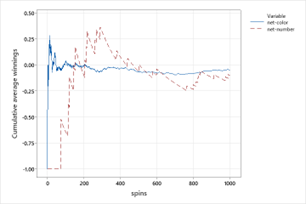
Below are two graphs showing the average net winnings over 1000 simulated plays of a color bet and of a number bet. [Hint: What happened on the first 50 or so number bets?] Explain how you think the expected value (long-run average winnings) of each bet compares. Do they have the same sign?

🔗

Graph showing cumulative average net winnings over 1000 simulated plays for color bet (blue line) and number bet (red dashed line)

Hint.

Look at where the graphs appear to be stabilizing as the number of plays increases. What does the long-run average appear to be approaching for each bet?

🔗

Checkpoint 1.2.34. Calculate Expected Values.

Explain which bet displays a larger standard deviation.

🔗

You have attempted of activities on this page.

🔗

Prev Top Next