Section 7.2 Investigation 2.5: Healthy Body Temperatures

Remark 7.2.1.

In the previous investigation, we assumed random sampling from a finite population to predict the distribution of sample means and help us evaluate whether a particular value is an unlikely value for the sample mean by chance alone. However, this method is not realistic in practice as we had to make up a population to sample from and we had to make some assumptions about that population (e.g., shape). Luckily, the Central Limit Theorem also predicts how that distribution would behave for most population shapes. But the CLT does require us to know certain characteristics about the population.

What is a healthy body temperature? German physician Carl Wunderlich analyzed a million temperatures from 25,000 patients and in 1869 published that the normal human-body temperature is 98.6Β°F. But several more recent studies have found that number to be too high, leading to speculation that Dr. Wunderlich was wrong, or that human body temperature has changed over time.
Introduction image for Healthy Body Temperatures investigation
In a study published by Mackowiak, Wasserman, & Levine (Journal of the American Medical Association, 1992), body temperatures (oral temperatures using a digital thermometer) were recorded for healthy men and women, aged 18-40 years, who were volunteers in Shigella vaccine trials at the University of Maryland Center for Vaccine Development, Baltimore. For these adults, the mean body temperature was found to be 98.249Β°F with a standard deviation of 0.733Β°F.

Checkpoint 7.2.2. Define symbols in context.

Explain (in words, in context) what is meant by the following symbols as applied to this study: \(n\text{,}\) \(\bar{x}\text{,}\) \(s\text{,}\) \(\mu\text{,}\) \(\sigma\text{.}\) If you know a value, report it. Otherwise, define the symbol in words.
\(n\) =
\(\bar{x}\) =
\(s\) =
\(\mu\) =
\(\sigma\) =
Solution.
\(n\) represents the number of people in the study (hasn’t been specified yet), \(\bar{x}\) = 98.249 = sample mean body temperature, \(s\) = 0.733 = sample standard deviation of the body temperatures, \(\mu\) = mean body temp in population (unknown), \(\sigma\) = standard deviation of body temperatures in entire population (unknown)

Checkpoint 7.2.3. Write hypotheses.

Write a null hypothesis and an alternative hypothesis for testing Wunderlich’s axiom using appropriate symbols.
\(H_0\text{:}\)
\(H_a\text{:}\)
Solution.
Let \(\mu\) represent the mean body temperature in the population of healthy adults.
\(H_0: \mu = 98.6\) (the body temperature of all healthy adults is 98.6)
\(H_a: \mu \neq 98.6\) (the body temperature of all healthy adults is no longer 98.6)

Checkpoint 7.2.4. Apply Central Limit Theorem.

Suppose the axiom is correct and many different random samples of 13 adults are taken from a large normally distributed population with mean 98.6Β°F. What does the Central Limit Theorem tell you about the theoretical distribution of sample means? (Indicate any necessary information that is missing.)
Solution.
The distribution of sample means will be normally distributed (because the population is) with a mean equal to 98.6 (our assumption for the mean body temperature of the population), and standard deviation \(\sigma/\sqrt{n}\text{.}\)
If we assume the null hypothesis is true, then we have a value to use for the population mean. However, we don’t have a value to use for the population standard deviation (sometimes called a "nuisance parameter" because we need its value to be able to use \(SD(\bar{x})\text{,}\) but it is not the parameter of interest).

Checkpoint 7.2.5. Estimate population standard deviation.

Suggest a method for estimating the population standard deviation from the sample data.
Solution.
We could use the sample standard deviation, \(s\text{.}\)

Definition: Standard Error of the Sample Mean.

The standard error of the sample mean, denoted by \(SE(\bar{x})\text{,}\) is an estimate of the standard deviation of \(\bar{x}\) (the sample to sample variability in sample means from repeated random samples) calculated by substituting the sample standard deviation \(s\) for the population standard deviation \(\sigma\text{:}\)
\begin{equation*} SE(\bar{x}) = \frac{s}{\sqrt{n}} \end{equation*}

Checkpoint 7.2.6. Calculate standard error.

Calculate the value of the standard error of the sample mean body temperature for this study when \(n = 13\text{.}\)
SE(\(\bar{x}\)) =
Solution.
\(s/\sqrt{n} = 0.733/\sqrt{13} \approx 0.203\)

Checkpoint 7.2.7. Calculate standardized statistic.

Determine how many standard errors the sample mean (98.249) falls from the hypothesized value of 98.6 (the standardized statistic).
standard errors
Solution.
\((98.249 - 98.6)/0.203 \approx -1.73\) standard errors

Checkpoint 7.2.8. Evaluate standardized statistic.

Based on this calculation, would you consider the value of the sample mean (98.249) to be surprising, if the population mean were really equal to 98.6? Explain how you are deciding.
Solution.
\(|-1.73|\) is less than 2 so doesn’t seem all that unusual for the sample mean when \(\mu = 98.6\text{.}\)
Previously, we compared our standardized statistics (\(z\)-scores) to the normal distribution and said (absolute) values larger than two were considered rare. But we don’t really have a \(z\)-score here because we had to estimate the standard deviation of the sample mean. This creates even more "uncertainty" in our standardized statistic and more random variation. Is that still true that two standard errors is unusual? Let’s explore the method you just used to standardize the sample mean in more detail.

Explore with simulation.

Open the Sampling from a Finite Population applet and paste the hypothetical population body temperature data from the BodyTempPop.txt file (or type the file name into the empty Population data window).

Checkpoint 7.2.9. Examine population distribution.

Does this appear to be a normally distributed population? What are the values of the population mean and the population standard deviation?
Solution.
Yes, the population distribution of body temperatures appears normally distributed with mean about 98.6 degrees and standard deviation 0.733 degrees.

Checkpoint 7.2.10. Verify Central Limit Theorem.

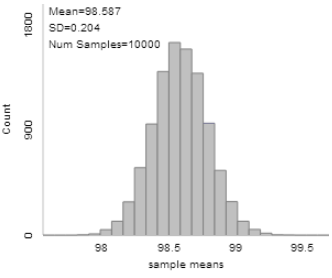
Use the applet to select 10,000 samples of 13 adults from this hypothetical population. Confirm that the behavior of the distribution of sample means is consistent with the Central Limit Theorem?
Hint.
Discuss shape, center, and variability; compare the CLT predictions to the simulation results.
Solution.
This is consistent with the central limit theorem as the shape is approximately normal, the mean is the same as the population mean, and the standard deviation is predicted by \(0.733/\sqrt{13} = 0.203\text{.}\)
Sampling distribution showing consistency with Central Limit Theorem
But what about the statistic suggested in Checkpoint 7.2.6; does this standardized statistic behave nicely and is this distribution again well modeled by a normal distribution?

Checkpoint 7.2.11. Examine \(t\)-statistic distribution.

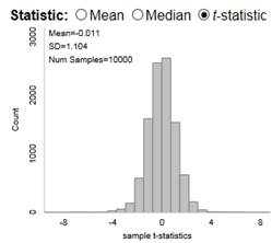
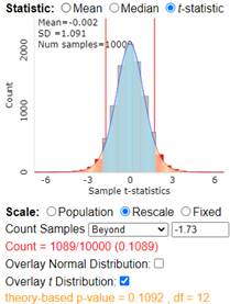
In the applet, change the Statistic option (above the graph) to \(t\)-statistic, the name for the standardized sample mean using the standard error of the sample mean. Describe the shape of the distribution of these \(t\)-statistics from your 10,000 random samples.
Solution.
The shape is symmetric and bell-shaped, with mean roughly zero and standard deviation a little larger than 1.
Distribution of t-statistics from 10,000 random samples

Checkpoint 7.2.12. Compare to normal distribution.

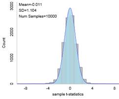
Check the box to Overlay Normal Distribution; does this appear to be a reasonable fit? What p-value does this normal approximation produce?
Hint.
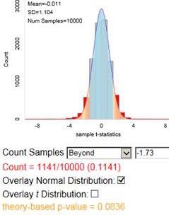
Enter your answer to Checkpoint 7.2.6 as the observed result for the \(t\)-statistic and count beyond.
Solution.
The fit seems good, but not perfect. The normal distribution is perhaps a bit too "skinny" in the middle and doesn’t go out far enough in the ends.
t-distribution with normal overlay showing fit comparison
p-value calculation using normal approximation

Checkpoint 7.2.13. Evaluate normal approximation.

Does the theory-based p-value from the normal distribution accurately predict how often we would simulate a standardized statistic at least as extreme (in either direction) as the observed value of 1.73? Does it over predict or underpredict?
Hint.
How does the behavior of the distribution of the standardized statistics most differ from a normal model?
Solution.
The normal distribution underpredicts how often the sample mean falls 1.73 SEs from the population mean.

Discussion.

If we zoom in on the tails of the distribution, we see that more of the simulated distribution lies in those tails than the normal distribution would predict.
Combined view of distribution tail comparisons
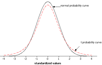
To model the sampling distribution of the standardized statistic \(\frac{\bar{x} - \mu}{s/\sqrt{n}}\text{,}\) we need a density curve with heavier tails than the standard normal distribution. William S. Gosset, a chemist turned statistician, showed in 1908, while working for the Guinness Breweries in Dublin, that a "t probability curve" provides a better model for the sampling distribution of this standardized statistic when the population of observations follows a normal distribution.

Checkpoint 7.2.14. Compare \(t\)-distribution to normal.

Check the Overlay \(t\)-distribution box. What is the main visual difference in the \(t\)-distribution model compared to the normal distribution model? Does this \(t\)-distribution appear to be a better model for the simulated sampling distribution? Is the theory-based p-value using the \(t\)-distribution closer to the empirical p-value than the theory-based p-value using the normal distribution?
Solution.
The \(t\) distribution has heavier tails, more area out there, giving us a better prediction. The p-value from the \(t\) distribution is much closer to the simulation results.

Checkpoint 7.2.15. Analyze with larger sample size.

The actual body temperature study involved a sample of \(n = 130\) adults. Use the applet to generate a sampling distribution of \(t\)-statistics for this sample size. Toggle between the normal and \(t\) probability distributions. Do you see much difference between them? What is the actual value of the observed \(t\)-statistic with this sample size? Where does it fall in this distribution? What do you conclude about the null hypothesis?
Solution.
With a sample size of 130, we don’t see as much distinction between the normal and \(t\) distributions. With \(n = 130\text{,}\) \(SE = 0.733/\sqrt{130} \approx 0.0643\) and \(t = (98.249 - 98.6)/0.0643 \approx -5.459\text{.}\) The sample mean of 98.249 is 5.459 standard errors below the population mean of 98.6, which implies 98.249 would be very surprising to observe for the sample mean if the population mean were really 98.6. This is far out in the tail of the simulated sampling distribution and gives strong evidence against the null hypothesis that the population mean is equal to 98.6. (We would reject the null hypothesis.)
Sampling distribution of t-statistics for n=130 with observed value

Discussion.

The consequence of this exploration is that when we are estimating both the population mean and the population standard deviation, we will compare our standardized statistic for the sample mean to the \(t\)-distribution instead of to the normal distribution to approximate p-values and confidence intervals. Although with larger sample sizes, the distinction will be quite minor.

Probability Detour – Student’s \(t\)-distribution.

The \(t\) probability density curve is described by the following function:
\begin{equation*} f(x) = \frac{\Gamma\left(\frac{\nu+1}{2}\right)}{\sqrt{\nu\pi}\,\Gamma\left(\frac{\nu}{2}\right)}\left(1+\frac{x^2}{\nu}\right)^{-\frac{\nu+1}{2}} \end{equation*}
where \(-\infty < x < \infty\)
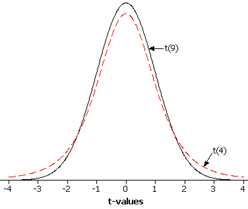
An impressive function indeed! But you should notice that this function only depends on the parameter \(\nu\text{,}\) referred to as the degrees of freedom.
This symmetric distribution has heavier tails than the standard normal distribution. We get a different \(t\)-distribution for each value of the degrees of freedom. As the degrees of freedom increase, the \(t\)-distribution approaches the standard normal distribution.
t-distribution curves with different degrees of freedom
t-distribution approaching normal distribution as degrees of freedom increase

One-sample \(t\)-test for \(\mu\).

To test a null hypothesis about a population mean \(H_0: \mu = \mu_0\text{,}\) when we don’t know the population standard deviation (pretty much always), we will use the sample standard deviation to calculate the standard error \(SE(\bar{x})\) and compare the standardized statistic
\begin{equation*} t = \frac{\bar{x} - \mu_0}{SE(\bar{x})} = \frac{\bar{x} - \mu_0}{s/\sqrt{n}} \end{equation*}
to a \(t\)-distribution with \(n - 1\) degrees of freedom. Theoretically, this approximation requires the population to follow a normal distribution. However, statisticians have found this approximation to also be reasonable for other population distributions whenever the sample size is large. How large the sample size needs to be depends on how skewed the population distribution is. Consequently, we will consider the \(t\) procedures valid when either the population distribution is symmetric or the sample size is large (e.g., larger than 30).

Probability Detour – Degrees of Freedom.

Recall the formula for the sample standard deviation \(s\) (Investigation A), compares each observed data value \(x_i\) to the sample mean \(\bar{x}\text{.}\) But \(\bar{x}\) is calculated by averaging those same data values. So if I know \(n - 1\) of those data values and I know \(\bar{x}\text{,}\) then that last observation is forced to be a particular value. So we say the calculation has \(n - 1\) degrees of freedom, and that’s why that formula divides by \(n - 1\text{.}\)

But what about confidence intervals?

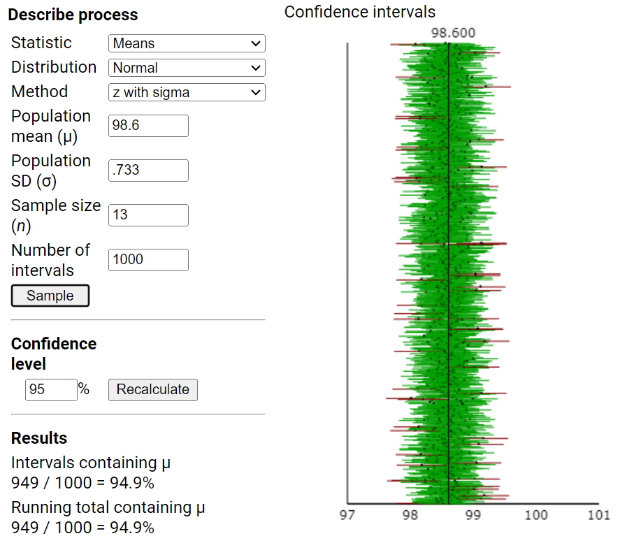
  • Change the Statistic to Means, but keep the Distribution set to Normal and the Method as \(z\) with sigma.
  • Set the population mean to 98.6, the population standard deviation to 0.733, and the sample size to 13.

Checkpoint 7.2.16. Examine \(z\) with sigma intervals.

Generate 1000 random samples from this population and examine the running total for the percentage of 95% confidence intervals \((\bar{x} \pm 1.96\sigma/\sqrt{n})\) that successfully capture the actual value of the population mean \(\mu\text{.}\)
  1. Is this 95% confident "\(z\) with sigma" procedure behaving as it should? How are you deciding?
  2. Press Sort. In what situations can an interval fail to capture \(\mu\text{?}\)
Solution.
Results will vary, but should be close to 95%, indicating that the method does achieve the claimed confidence level. After sorting, we can see that intervals fail to capture \(\mu\) when the sample mean is unusually far from the population mean.
Confidence interval simulation showing 95% coverage rate

Checkpoint 7.2.17. Predict effect of using \(s\).

But more realistically, we don’t know \(\sigma\) and will use \(s\) in calculating our confidence interval (\(\bar{x} \pm 1.96s/\sqrt{n}\)). Predict what will change about the resulting confidence intervals from different random samples if we use each sample standard deviation in place of \(\sigma\text{.}\)
Hint.
Think of two main properties of confidence intervals.
Solution.
Predictions will vary, but should think about how lengths of intervals will change from sample to sample. (The centers will be the same for both CI simulations.)

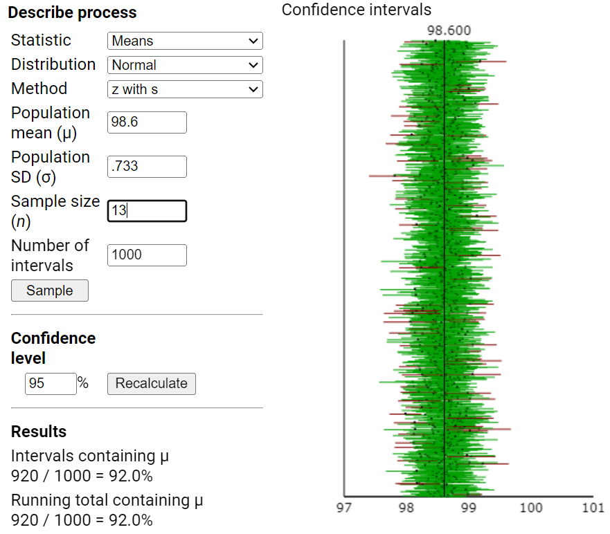
Checkpoint 7.2.18. Test \(z\) with \(s\) method.

Change the Method now to \(z\) with \(s\text{.}\) What percentage of these 1000 confidence intervals succeed in capturing the population mean of 98.6? Is this close to 95%? If not, is it larger or smaller?
Solution.
Percentage drops to 91 or 92%.
Confidence interval simulation using z with s method showing reduced coverage

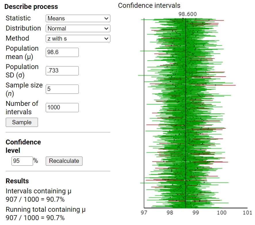
Checkpoint 7.2.19. Repeat with smaller sample size.

Repeat the previous question with a sample size of \(n = 5\text{.}\)
Solution.
With a sample size of 5, the percentage will be closer to or even below 90% indicating that the method does not work as it should.
Confidence interval simulation with n=5 showing poor coverage rate

Discussion.

This "\(z\) with \(s\)" procedure produces a coverage rate (for successfully capturing the value of the population mean) that is less than 95%, because again the normal distribution doesn’t account for the additional uncertainty resulting from sample to sample when we need to use both \(\bar{x}\) and \(s\text{.}\) The fix will be to multiply the standard error by a critical value larger than 1.96 to compensate for the additional uncertainty introduced by estimating \(\sigma\) with \(s\text{.}\) The \(t\)-distribution will come to our rescue. Which \(t\)-distribution do we use? That will depend on our sample size; with smaller samples we need heavier tails and with larger samples we need a distribution more like the normal probability model. The heaviness of the tails will be determined by the "degrees of freedom" of the \(t\)-distribution.

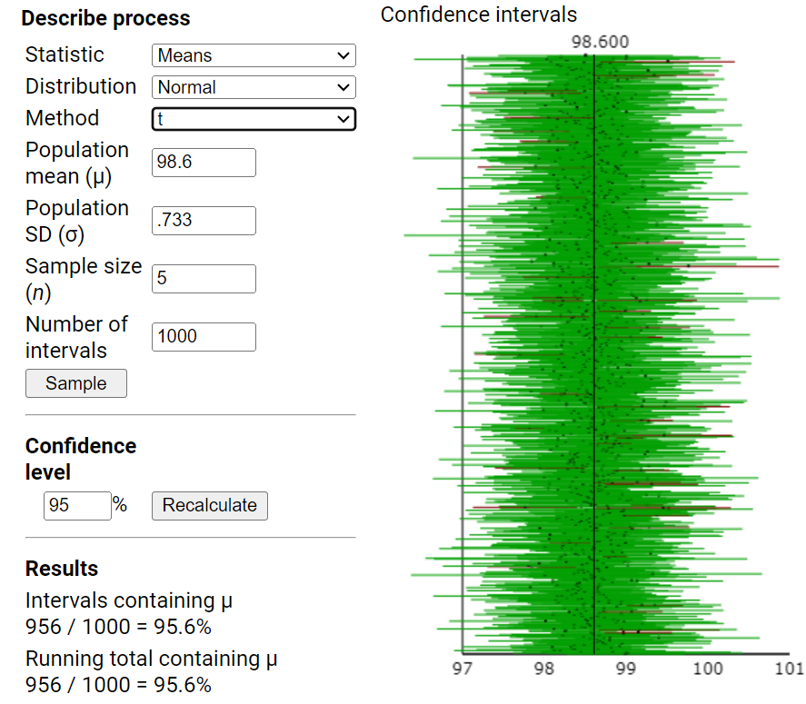
Checkpoint 7.2.20. Test \(t\)-interval method.

Change the Method to t. How do the intervals visibly change? Is the coverage rate indeed closer to 95%?
Solution.
The intervals become longer and now the overall percentage is closer to 95%.
Confidence interval simulation using t method showing improved coverage
This leads to a confidence interval formula with the same general form as in the previous chapter: \(sample\ statistic \pm (critical\ value) \times (SE\ of\ statistic)\text{,}\) where the critical value now comes from the \(t_{n-1}\) distribution (degrees of freedom = \(n - 1)\) instead of from the standard normal distribution.

One-sample \(t\)-interval for \(\mu\).

When we have a symmetric sample or a large sample size, an approximate confidence interval for \(\mu\) is given by:
\begin{equation*} \bar{x} \pm t_{n-1}^* \times \frac{s}{\sqrt{n}} \end{equation*}
Keep in mind that the critical value \(t^*\) tells us how many standard errors we need to extend from the sample mean (in each direction) based on how confident we want to be. Our goal is to develop a \(100 \times C\%\) confidence interval method that will capture the population parameter \((100 \times C)\%\) of the time in the long run.

Technology Detour β€” Finding \(t^*\).

Checkpoint 7.2.21. \(t\) Probability Calculator applet.

Using the \(t\) Probability Calculator applet below:
  1. Specify the degrees of freedom
  2. Check the box next to the less than symbol and then enter \((1-C)/2\) (e.g., 0.025 for 95% confidence) in the probability box and press Return. The \(t\)-value box should fill in.

Checkpoint 7.2.22. Finding \(t^*\) with R.

Assuming 95% confidence with df = 4:
iscaminvt(.95, 4, "between")

Checkpoint 7.2.23. Finding \(t^*\) with JMP.

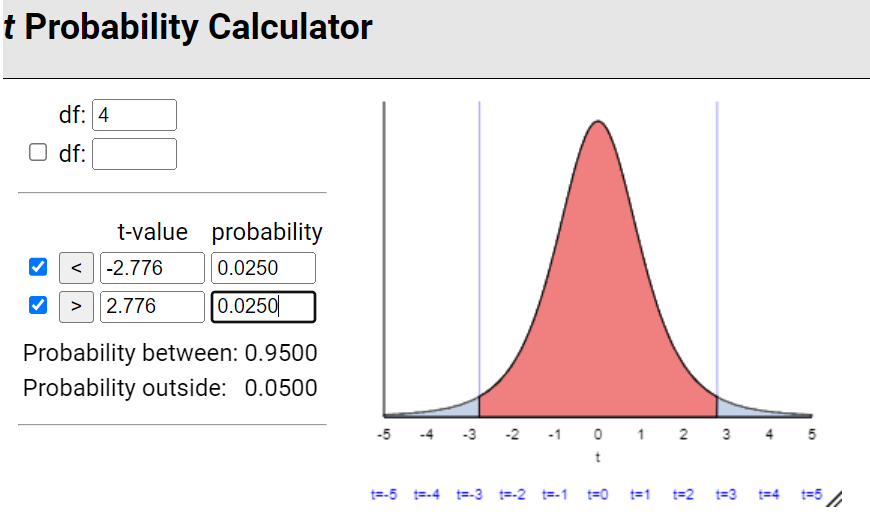
Checkpoint 7.2.24. Find \(t^*\) for \(n\ =\ 5\).

Using one of the above technology detours, find the \(t^*\) value corresponding to a 95% confidence level and a sample size of \(n = 5\text{.}\)
\(t_4^*\) =
Solution.
\(t_4^* = 2.776\)
t probability calculator showing t* value for df=4

Checkpoint 7.2.25. Compare \(t^*\) to \(z^*\).

How does the \(t^*\) critical value of 2.776 compare to the corresponding \(z^*\) value of 1.96 for 95% confidence?
  • Smaller
  • No change
  • Larger

Checkpoint 7.2.26. Find \(t^*\) for \(n = 13\).

Find the \(t^*\) value for the sample size of \(n = 13\text{.}\) How do the \(t\)-critical values compare for these different sample sizes? Is this what you expected? Explain.
Solution.
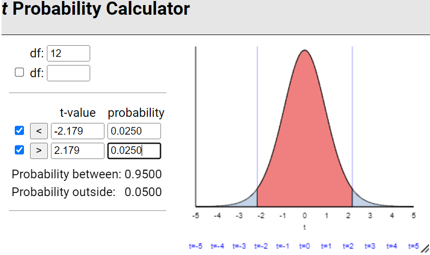
The t critical value of 2.179 is much closer to the z critical value of 1.96 with a larger sample size. Compared to the \(t\) critical value from Checkpoint 7.2.20, the current critical value has decreased suggesting that the t critical value will approach the \(z\) critical value as the sample size increases. (By \(n = 130\text{,}\) \(t^* = 1.98\text{.}\))
t probability calculator showing t* value for df=12

Checkpoint 7.2.27. Find \(t^*\) for \(n = 130\).

Find \(t^*\) for the sample size of \(n = 130\text{.}\)
\(t_{129}^*\) =
How does this value compare to the earlier \(t^*\) values?
How does this value compare to the \(z^*\) value?
Solution.
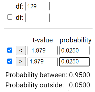
For \(n = 130\) (df = 129), \(t^* = 1.979\text{,}\) getting pretty close to 1.96. As the sample size increases, the \(t^*\) value decreases and approaches the \(z^*\) value.
t probability calculator showing t* value for df=129

Checkpoint 7.2.28. Calculate confidence interval.

Use the critical value from the previous question to calculate a 95% confidence interval for the mean body temperature of a healthy adult based on our sample \((\bar{x} = 98.249\text{,}\) \(s = 0.733\text{,}\) \(n = 130)\text{.}\) Is this interval consistent with your conclusion about the null hypothesis in Checkpoint 7.2.14? Explain.
Solution.
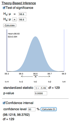
95% confidence interval = \(98.249 \pm 1.979 \times \frac{0.733}{\sqrt{130}} = 98.249 \pm 0.127 = (98.122, 98.376)\text{.}\) This interval does not contain 98.6, which is consistent with our rejection of 98.6 as a plausible value for the population mean.

Technology Detour β€” One Sample \(t\)-procedures.

Checkpoint 7.2.29. One Sample \(t\) with Theory-Based Inference applet.

  1. Select One mean from the Scenario pull-down menu
  2. You can check Paste data to copy and paste in the raw data, or type in the sample size, mean, and standard deviation. Press Calculate.
  3. Check the box for Test of significance and enter the hypothesized value of \(\mu\) and set the direction of the alternative. Press Calculate.
  4. Check the box for Confidence interval, enter the confidence level and press Calculate CI.
Solution.
Here are the steps illustrated:
Step 1: Entering data in Theory-Based Inference applet
Step 2: Setting up hypothesis test
Step 3: Calculating confidence interval
described in detail following the image
Theory-Based Inference applet output for one sample \(t\)-test and confidence interval

Checkpoint 7.2.30. One Sample \(t\) with R.

You can use the t.test command with raw data ("x") or iscamonesamplet with summary data:
t.test(x, mu = hypothesized_value, alternative="two.sided", conf.level = .95)
iscamonesamplet(xbar=98.249, sd=.733, n=130, hypothesized=98.6, 
                alternative="two.sided", conf.level=95)
where sd = sample standard deviation, \(s\text{.}\)
Solution.

Checkpoint 7.2.31. One Sample \(t\) with JMP.

You can use raw data or summary data (see second option):
  1. In the Data window, choose Analyze > Distribution
  2. Specify the variable in the Y, Columns box
  3. The 95% confidence interval will be shown in the Summary Statistics box. If you want to change the confidence level, use the variable hot spot and select Confidence interval.
  4. To perform the test of significance, use the variable hot spot, select Test Mean. Then enter the hypothesized value of \(\mu\) and press OK.
  1. Open the ISCAM Journal file > Hypothesis Test for One Mean
  2. Choose Raw Data (and pick the column) or Summary Statistics (and then specify the sample size, sample mean, and sample standard deviation)
  3. Be sure to choose the \(t\)-test Test Type and specify the alternative hypothesis
  4. In the ISCAM Journal file > Confidence Interval for One Mean
  5. Choose the \(t\) interval type and specify confidence level
Solution.

Checkpoint 7.2.32. Use technology to verify calculations.

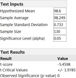
Use technology to verify your by-hand calculations and summarize the conclusions you would draw from this study (both from the p-value and the confidence interval, including the population you are willing to generalize to). Also include interpretations, in context, of your p-value and your confidence level.

Study Conclusions.

The sample data provide very strong evidence that the mean body temperature of healthy adults is not 98.6 degrees (\(t = 5.46\text{,}\) two-sided p-value \(< 0.001\)). This indicates there is less than a 0.1% chance of obtaining a sample mean as far from 98.6 as 98.249 in a random sample of 130 healthy adults from a population with mean body temperature of 98.6 Β°F. A 95% confidence interval for the population mean body temperature is (98.122, 98.376), so we can be 95% confident that the population mean body temperature among healthy adults is between 98.122 and 98.376 Β°F. This interval is entirely less than 98.6, consistent with our having found very strong evidence to reject 98.6 as a plausible value for the population mean. We are 95% confident, meaning if we were to repeat this procedure on thousands of random samples, in the long-run roughly 95% of the resulting intervals would successfully capture the population mean. We believe these procedures are valid because the sample size of 130 should be large enough unless there is severe skewness in the population.

Subsection 7.2.1 Practice Problem 2.5A

Explore the last statements in the above results box using \(t\) confidence intervals:

Checkpoint 7.2.33. Coverage rate for skewed population.

Continue with the Simulating Confidence Intervals applet. Simulating Confidence Intervals applet. Explore the coverage rate of the \(t\)-procedure with random samples from an Exponential (skewed) population for \(n = 5\text{,}\) \(n = 100\text{,}\) and \(n = 200\text{.}\) Assess and summarize the performance of this \(t\)-procedure in each case.

Checkpoint 7.2.34. Coverage rate for uniform population.

Repeat the previous question for a Uniform population distribution with endpoints \(a = 80\) and \(b = 85\text{.}\)

Subsection 7.2.2 Practice Problem 2.5B

Stanford researchers (e.g., Protsiv et al., 2020) claim that average normal human-body temperature is closer to 97.5 degrees Fahrenheit (McGinty, Wall Street Journal, 2020). Part of the Stanford study was to use digital oral instruments to take temperature readings from 150,280 individuals 2007-2017 (578,222 measurements). They found a mean of 98.04 Β°F and a standard deviation of 0.502 Β°F.

Checkpoint 7.2.35. Interpret standard deviation.

Provide a one-sentence interpretation of the standard deviation.

Checkpoint 7.2.36. Sources of variation.

Identify some "sources of variation" in individual body temperatures. Which of these are "between individuals" and which are "within individuals"?

Checkpoint 7.2.37. Source not captured by SD.

Identify a source of variation in temperature measurements not captured by the standard deviation.

Checkpoint 7.2.38. Justify \(t\)-distribution.

Give two reasons why a \(t\) [Hint: Click on the slider handle and use the arrow keys on your keyboard.] -distribution is likely to be an appropriate model for these data.

Checkpoint 7.2.39. Test temperature claim.

Using the mean and SD values provided, do these data provide convincing evidence that the average healthy body temperature is below 98.6 Β°F? Comment on both a p-value and a 95% confidence interval.

Checkpoint 7.2.40. Define high temperature.

Based on these data, what would you consider a statistically high body temperature for an individual?

Checkpoint 7.2.41. Evaluate Wunderlich’s measurements.

From this analysis can we conclude that Wunderlich’s measurements were flawed? What could be another explanation?

Subsection 7.2.3 Practice Problem 2.5C

Checkpoint 7.2.42. Evaluate observed mean.

As in Checkpoint 7.2.9, use the Sampling from Finite Population applet to select 10,000 samples of 13 adults from the hypothetical population of 10,000 body temperatures. Based on the generated distribution of sample means, is the observed mean of 98.249 (or more extreme in either direction) a surprising outcome for this population?

Checkpoint 7.2.43. Find interval of plausible values.

Check the Fixed radio button and use the Shift center slider on the left-hand side to (slowly) raise the population mean. Stop when you find a value of the population mean that you first consider surprising. Now use the slider to lower the population mean. What is the smallest value for \(\mu\) that you consider plausible based on this sample mean? In other words, report your interval of plausible values.
Hint.
Click on the slider handle and use the arrow keys on your keyboard.

Checkpoint 7.2.44. Repeat for \(n = 130\).

You have attempted of activities on this page.