Statistician Jessica Utts has conducted extensive analysis of studies that have investigated psychic functioning. (Combining results across multiple studies, often to increase power, is called meta-analysis.) Utts (1995) cites research from Bem and Honorton (1994) that analyzed studies that used a technique called ganzfeld.
In a typical ganzfeld experiment, a "receiver" is placed in a room relaxing in a comfortable chair with halved ping-pong balls over the eyes, having a red light shone on them. The receiver also wears a set of headphones through which [static] noise is played. The receiver is in this state of mild sensory deprivation for half an hour. During this time, a "sender" observes a randomly chosen target and tries to mentally send this information to the receiver … The receiver is taken out of the ganzfeld state and given a set of [four] possible targets, from which they must decide which one most resembled the images they witnessed. Most commonly there are three decoys along with a copy of the target itself. [Wikipedia]
Suppose you want to test whether the subjects in these studies have ESP, with \(\pi\) equal to the actual probability that receivers identify the correct image among the four possible targets. State appropriate null and alternative hypotheses by specifying correct symbols and values.
Checkpoint3.5.2.Check CLT and Describe Null Distribution.
The Bem and Honorton study reports on 329 sessions. Is this a large enough sample size to employ the Central Limit Theorem? Report the predicted mean and standard deviation of the null distribution of sample proportions.
We expect the distribution of sample proportions to be approximately normal with mean \(\mu_{\hat{p}} = 0.25\) and standard deviation \(\text{SD}(\hat{p}) = \sqrt{\frac{0.25(0.75)}{329}} \approx 0.02387\text{.}\)
In Investigation 1.3, you determined that if someone was asked to choose among 5 symbols in 10 rounds, they would need to correctly identify 5 or more of the symbols to produce a p-value below 0.05 and be at least two standard deviations away from the expected 2 correct identifications. The result "5 or more correct" is often called the rejection region (the values of the statistic that lead us to reject the null hypothesis).
The rejection region consists of the values we would need to observe for the statistic in the study in order to be willing to reject the null hypothesis.
According to the distribution in Checkpoint 2, what proportion of the 329 sessions would need to be successful ("hits"), in order to reject the null hypothesis in Checkpoint 1 in favor of the alternative hypothesis at the 5% level of significance?
A Type I error in a test of significance occurs when the null hypothesis is true but we decide to reject the null hypothesis. This type of error is sometimes referred to as a false positive or a "false alarm."
According to the applet, what is the (normal approximation) probability of making a Type I error in this study? How could you have known this in advance? (Note that the normal approximation is not required to correspond to an integer value for the rejection region.)
While a Type I error focuses on the null hypothesis being true, what if the null hypothesis is false – how likely are we to make the correct decision to reject the null hypothesis?
A Type II error occurs when we fail to reject the null hypothesis even though the null hypothesis is false. This type of error is sometimes referred to as a false negative or a "missed opportunity."
The power of a test when \(\pi = \pi_a\) is defined as the probability of (correctly) rejecting the null hypothesis assuming this specific alternative value for the parameter. Thus, power reveals how likely our test is to detect a specific difference (or improvement or effect) that really is there.
Checkpoint3.5.5.Describe Alternative Distribution.
Suppose the probability of identifying the correct symbol is actually 0.30. Describe how the distribution of sample proportions will differ from Checkpoint 2.
If we test \(\pi = 0.25\) but in reality \(\pi = 0.30\text{,}\) we will correctly reject the null hypothesis in favor of the one-sided alternative in about 66% of random samples of size n = 329. So the power of this test is approximately 0.66.
Now find the probability of rejecting the null hypothesis that \(\pi = 0.25\) when in reality \(\pi = 0.35\text{?}\) Explain your steps. How has the probability changed and why?
If the alternative value changes to 0.35, then the power increases to about 0.99. This makes sense because when the true parameter is farther from the null hypothesis value (0.35 vs 0.30), it becomes easier to detect the difference, so we have a higher probability of correctly rejecting the null hypothesis.
Checkpoint3.5.9.Small Sample Size with Exact Binomial.
Suppose the study had only involved 35 sessions. Because the sample size is small, use of the Central Limit Theorem is questionable. Uncheck the Normal Approximation box and check the Exact Binomial box. Specify a hypothesized probability of 0.25, an alternative probability of 0.35, and a level of significance of 0.05. Report the following:
Checkpoint3.5.10.Compare Power for Different Sample Sizes.
How does the power in Checkpoint 9 compare to what you found for power earlier? [Hint: see Checkpoint 7] Explain why this relationship makes intuitive sense.
The power is much smaller with the smaller sample size (about 32% vs 99%). This makes sense as there will be more sample-to-sample variation by chance alone with the smaller sample size, making it more difficult to distinguish observations coming from the two different distributions. In other words, there is more overlap in the two distributions and the probability of finding a sample proportion to convince us to reject the null hypothesis is smaller.
should reveal both distributions and report the rejection region to achieve the level of significance, the observed level of significance, and the power.
Specify the form of the alternative, the level of significance (Alpha), an alternative probability of success, and set the Test Method to Normal Approximation.
In fact, the most common application is to specify the desired power and solve for the necessary sample size before conducting the study to determine how many observations you should take.
Checkpoint3.5.13.Sample Size for 80% Power at π = 0.30.
If your technology allows (or use trial and error), see how many sessions would be needed in the ganzfeld study to have at least an 80% chance of rejecting the null hypothesis if the actual probability of success is \(\pi = 0.30\text{.}\)
Checkpoint3.5.14.Sample Size for 80% Power at π = 0.35.
How will your answer to (k) change if the actual probability of success is \(\pi = 0.35\text{?}\) Determine the number of sessions needed in this case.
If the actual probability of success is even further away from the hypothesized value (0.35 vs 0.30), then we won’t need as large a sample size to achieve the same power. The effect size is larger, making it easier to detect the difference with fewer observations.
We control the probability of a Type I error by stating a level of significance before we collect any data. We chiefly control the probability of a Type II error by determining what sample size is needed in a study to achieve a desired level of power. To do so, you need to establish in advance how false you think the null hypothesis is/what size of a difference you want to be able to detect. This is often done through subject-matter knowledge or prior study results.
If the researchers believe there is a genuine but small effect (say 5 percentage points) of ESP, then with a sample size of 329, there is about a 65% chance that, when the probability of a correct identification equals 0.30, they will obtain a sample result that convinces them to reject the null hypothesis that \(\pi = 0.250\text{.}\) With a sample size of around 500, there is over 80% chance that the researchers will find evidence of ESP when \(\pi = 0.30\text{.}\) Keep in mind that with a large sample size, we can often find a statistically significant result that we may not consider practically significant.
Discussion: When the sample size is small, the binomial distribution can be used for power calculations, but notice that the discreteness of the binomial probability distribution can complicate matters. This is another example where the normal distribution is simpler, but do keep in mind use of the normal approximation is not always valid.
For the research study on the mortality rate at St. George’s hospital (Investigation 1.4), the goal was to compare the mortality rate of that hospital to the national benchmark of 0.15.
Checkpoint3.5.15.Identify Type of Error (Exceeding Benchmark).
If you were to conclude that the hospital’s death rate exceeds the national benchmark when it really does not, what type of error would you be committing?
Checkpoint3.5.16.Identify Type of Error (Not Exceeding Benchmark).
If you were to conclude that the hospital’s death rate does not exceed the national benchmark when it really does, which type of error would you be committing?
A Type II error might be considered more critical because failing to detect that the hospital has a higher death rate than the benchmark means patients may continue to receive substandard care. However, a Type I error could also be serious as it might unfairly damage the hospital’s reputation. The answer may depend on the consequences of each type of error.
Checkpoint3.5.18.Compare Power for Different Alternatives.
Suppose you wanted to know the power of the test when the mortality rate at this hospital was 0.20 and when the mortality rate at this hospital was 0.25. For which alternative probability would you have a lower chance of committing a Type II error? Explain.
You would have a lower chance of committing a Type II error when \(\pi = 0.25\text{.}\) The power is higher when the true parameter value is further from the null hypothesis value (0.25 is further from 0.15 than 0.20 is), making it easier to detect the difference and reject the null hypothesis. Higher power means lower probability of Type II error.
Checkpoint3.5.19.Compare Type I Error Probabilities.
If Abe were to use a significance level of 0.05 and Bianca were to use a significance level of 0.01, who would have a smaller probability of Type I error? Explain briefly.
Bianca would have a smaller probability of Type I error. The probability of a Type I error equals the significance level, so Bianca’s probability (0.01) is smaller than Abe’s (0.05).
Checkpoint3.5.20.Compare Type II Error Probabilities.
If Abe were to use a significance level of 0.05 and Bianca were to use a significance level of 0.01, who would have a smaller probability of Type II error? Explain briefly.
Abe would have a smaller probability of Type II error. With a less stringent significance level (0.05 vs 0.01), it’s easier to reject the null hypothesis, which means higher power and therefore lower probability of Type II error.
Checkpoint3.5.21.Compare Type I Error with Different Sample Sizes.
If Abe were to use a significance level of 0.05 with a sample size of \(n = 50\) and Bianca were to use a significance level of 0.01 with a sample size of \(n = 100\text{,}\) who would have a smaller probability of a Type I error?
Bianca would have a smaller probability of Type I error. The probability of Type I error is determined solely by the significance level (not by sample size), and Bianca’s significance level (0.01) is smaller than Abe’s (0.05).
Checkpoint3.5.22.Compare Power with Different Sample Sizes.
If Abe were to use a significance level of 0.05 with a sample size of \(n = 50\) and Bianca were to use a significance level of 0.01 with a sample size of \(n = 100\text{,}\) whose test would have more power?
This depends on the specific alternative being considered, but in general, Bianca’s test might have more power despite the lower significance level, because her larger sample size (100 vs 50) substantially increases power. However, Abe’s higher significance level also increases power. The net effect would depend on the specific parameter values.
For the research study on the mortality rate at St. George’s hospital (Investigation 1.4), the goal was to decide whether the mortality rate of that hospital exceeds the national benchmark of 0.15. Suppose you plan to monitor the next 20 operations, using a level of significance of 0.05. Also suppose the actual death rate at this hospital equals 0.20.
Suppose you want to test a person’s ability to discriminate between two types of soda. You fill one cup with Soda A and two cups with Soda B. The subject tastes all 3 cups and is asked to identify the odd soda. You record the number of correct identifications in 10 attempts. Assume level of significance \(\alpha = 0.05\) and a one-sided alternative.
If the subject’s actual probability of a correct identification is 0.50, what is the power of this test for a level of significance of \(\alpha = 0.05\text{?}\)
The null hypothesis is \(\pi = 1/3\) (guessing among 3 cups). Use technology with \(n = 10\text{,}\)\(\pi_0 = 1/3\text{,}\)\(\pi_a = 0.50\text{,}\) and \(\alpha = 0.05\text{.}\)
If the subject can correctly identify the odd soda 50% of the time, there is approximately a 38% chance that we will correctly reject the null hypothesis (that they are just guessing) with 10 trials at the 0.05 significance level.
With \(n = 20\text{,}\) the power increases to approximately 0.63. The larger sample size makes it easier to detect the subject’s ability if they truly can identify the odd soda 50% of the time.
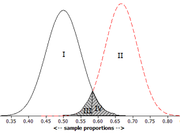
Suppose that you want to re-conduct the kissing study in a large city with a sample of 100 kissing couples. You want to test the null hypothesis \(H_0: \pi = 0.667\) against a one-sided alternative \(H_a: \pi < 0.667\) using a significance level of \(\alpha = 0.05\text{,}\) and you are concerned about the power of your test when \(\pi = 0.5\text{.}\)
Region I represents the Type I error probability - the area in the left tail of the null distribution (centered at 0.667) that falls in the rejection region.
Region II represents the Type II error probability - the area under the alternative distribution (centered at 0.5) that does not fall in the rejection region.
The table below shows the possible states of the world and the possible decisions we can make. Indicate where the types of errors fall in this table and where the test makes the correct decision.
sol1.png)
sol1.png)
sol2.png)
sol.png)
sols.png)
Rsol.jpg)
JMPsol.png)
Appletsol.jpg)